The following tutorial contains Python examples for solving regression problems. You should refer to the Appendix chapter on regression of the “Introduction to Data Mining” book to understand some of the concepts introduced in this tutorial. The notebook can be downloaded from http://www.cse.msu.edu/~ptan/dmbook/tutorials/tutorial5/tutorial5.ipynb.
Regression is a modeling technique for predicting quantitative-valued target attributes. The goals for this tutorial are as follows: 1. To provide examples of using different regression methods from the scikit-learn library package. 2. To demonstrate the problem of model overfitting due to correlated attributes in the data. 3. To illustrate how regularization can be used to avoid model overfitting.
Read the step-by-step instructions below carefully. To execute the code, click on the corresponding cell and press the SHIFT-ENTER keys simultaneously.
Synthetic Data Generation
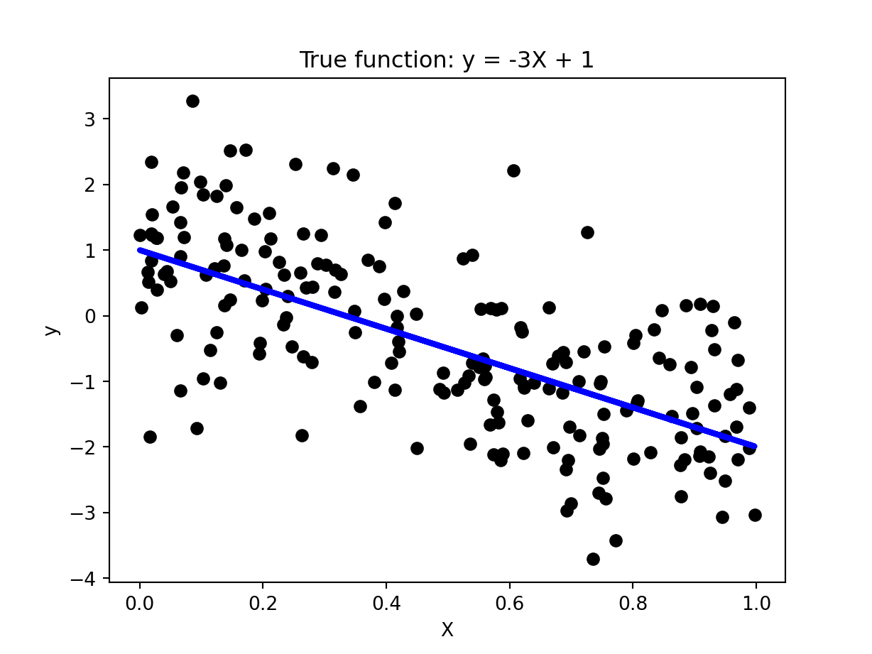
To illustrate how linear regression works, we first generate a random 1-dimensional vector of predictor variables, x, from a uniform distribution. The response variable y has a linear relationship with x according to the following equation: y = -3x + 1 + epsilon, where epsilon corresponds to random noise sampled from a Gaussian distribution with mean 0 and standard deviation of 1.
import numpy as npimport matplotlib.pyplot as pltseed =1# seed for random number generation numInstances =200# number of data instancesnp.random.seed(seed)X = np.random.rand(numInstances,1).reshape(-1,1)y_true =-3*X +1y = y_true + np.random.normal(size=numInstances).reshape(-1,1)plt.scatter(X, y, color='black')plt.plot(X, y_true, color='blue', linewidth=3)plt.title('True function: y = -3X + 1')plt.xlabel('X')plt.ylabel('y')plt.show()
Multiple Linear Regression
In this example, we illustrate how to use Python scikit-learn package to fit a multiple linear regression (MLR) model. Given a training set \({X,y}\) MLR is designed to learn the regression function \(f(X,w) = X^T w + w_0\) by minimizing the following loss function given a training set \(\{X_i,y_i\}_{i=1}^N\):
where \(w\) (slope) and \(w_0\) (intercept) are the regression coefficients.
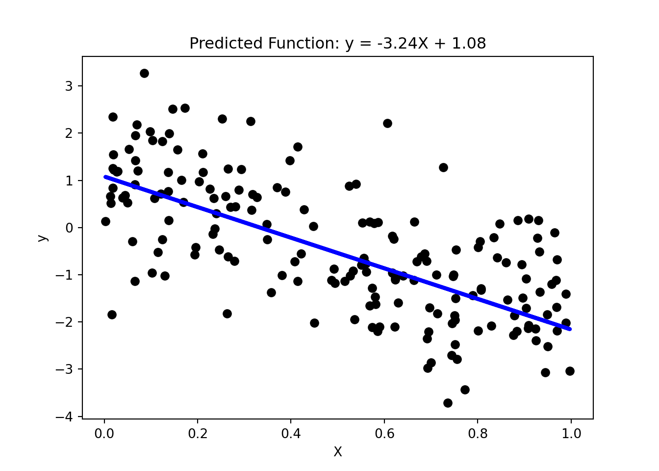
Given the input dataset, the following steps are performed: 1. Split the input data into their respective training and test sets. 2. Fit multiple linear regression to the training data. 3. Apply the model to the test data. 4. Evaluate the performance of the model. 5. Postprocessing: Visualizing the fitted model.
Step 1: Split Input Data into Training and Test Sets
numTrain =20# number of training instancesnumTest = numInstances - numTrainX_train = X[:-numTest]X_test = X[-numTest:]y_train = y[:-numTest]y_test = y[-numTest:]
Step 2: Fit Regression Model to Training Set
from sklearn import linear_modelfrom sklearn.metrics import mean_squared_error, r2_score# Create linear regression objectregr = linear_model.LinearRegression()# Fit regression model to the training setregr.fit(X_train, y_train)
LinearRegression()
In a Jupyter environment, please rerun this cell to show the HTML representation or trust the notebook. On GitHub, the HTML representation is unable to render, please try loading this page with nbviewer.org.
LinearRegression()
Step 3: Apply Model to the Test Set
# Apply model to the test sety_pred_test = regr.predict(X_test)
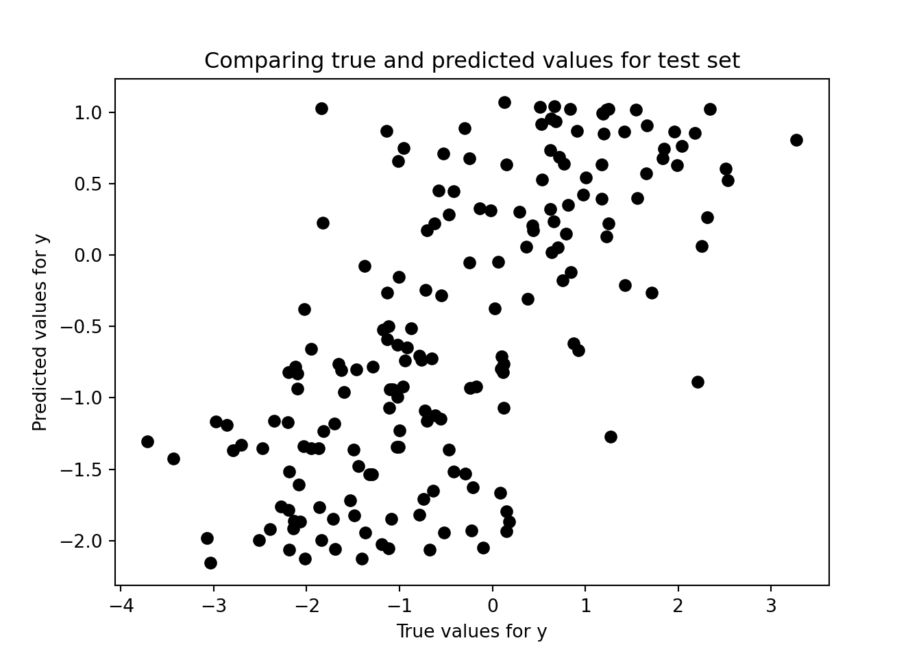
Step 4: Evaluate Model Performance on Test Set
# Comparing true versus predicted valuesplt.scatter(y_test, y_pred_test, color='black')plt.title('Comparing true and predicted values for test set')plt.xlabel('True values for y')plt.ylabel('Predicted values for y')# Model evaluationprint("Root mean squared error = %.4f"% np.sqrt(mean_squared_error(y_test, y_pred_test)))
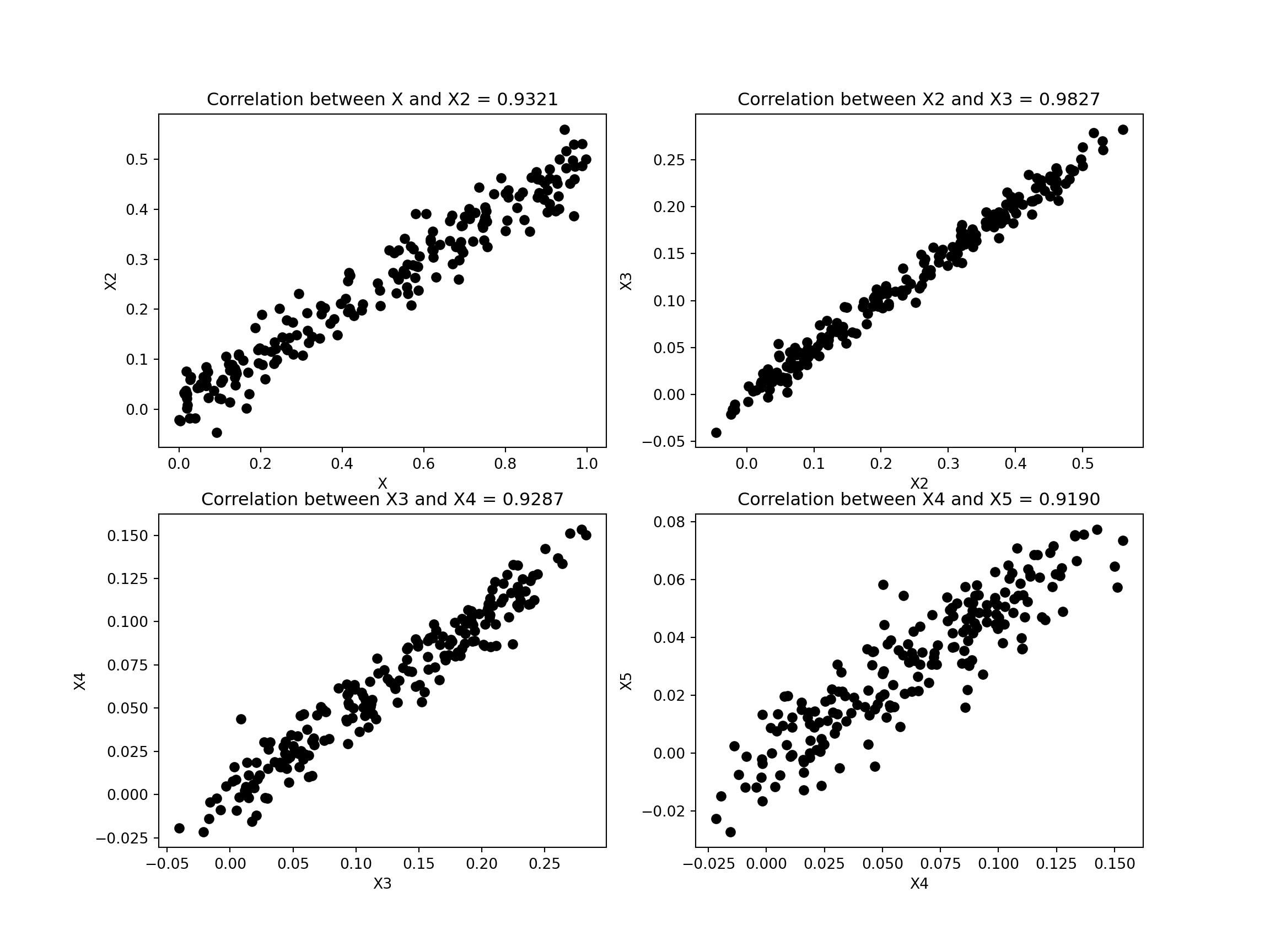
In this example, we illustrate how the presence of correlated attributes can affect the performance of regression models. Specifically, we create 4 additional variables, X2, X3, X4, and X5 that are strongly correlated with the previous variable X created in Section 5.1. The relationship between X and y remains the same as before. We then fit y against the predictor variables and compare their training and test set errors.
First, we create the correlated attributes below.
seed =1np.random.seed(seed)X2 =0.5*X + np.random.normal(0, 0.04, size=numInstances).reshape(-1,1)X3 =0.5*X2 + np.random.normal(0, 0.01, size=numInstances).reshape(-1,1)X4 =0.5*X3 + np.random.normal(0, 0.01, size=numInstances).reshape(-1,1)X5 =0.5*X4 + np.random.normal(0, 0.01, size=numInstances).reshape(-1,1)fig, ((ax1, ax2),(ax3,ax4)) = plt.subplots(2, 2, figsize=(12,9))ax1.scatter(X, X2, color='black')ax1.set_xlabel('X')ax1.set_ylabel('X2')c = np.corrcoef(np.column_stack((X[:-numTest],X2[:-numTest])).T)titlestr ='Correlation between X and X2 = %.4f'% (c[0,1])ax1.set_title(titlestr)ax2.scatter(X2, X3, color='black')ax2.set_xlabel('X2')ax2.set_ylabel('X3')c = np.corrcoef(np.column_stack((X2[:-numTest],X3[:-numTest])).T)titlestr ='Correlation between X2 and X3 = %.4f'% (c[0,1])ax2.set_title(titlestr)ax3.scatter(X3, X4, color='black')ax3.set_xlabel('X3')ax3.set_ylabel('X4')c = np.corrcoef(np.column_stack((X3[:-numTest],X4[:-numTest])).T)titlestr ='Correlation between X3 and X4 = %.4f'% (c[0,1])ax3.set_title(titlestr)ax4.scatter(X4, X5, color='black')ax4.set_xlabel('X4')ax4.set_ylabel('X5')c = np.corrcoef(np.column_stack((X4[:-numTest],X5[:-numTest])).T)titlestr ='Correlation between X4 and X5 = %.4f'% (c[0,1])ax4.set_title(titlestr)
Next, we create 4 additional versions of the training and test sets. The first version, X_train2 and X_test2 have 2 correlated predictor variables, X and X2. The second version, X_train3 and X_test3 have 3 correlated predictor variables, X, X2, and X3. The third version have 4 correlated variables, X, X2, X3, and X4 whereas the last version have 5 correlated variables, X, X2, X3, X4, and X5.
In a Jupyter environment, please rerun this cell to show the HTML representation or trust the notebook. On GitHub, the HTML representation is unable to render, please try loading this page with nbviewer.org.
In a Jupyter environment, please rerun this cell to show the HTML representation or trust the notebook. On GitHub, the HTML representation is unable to render, please try loading this page with nbviewer.org.
In a Jupyter environment, please rerun this cell to show the HTML representation or trust the notebook. On GitHub, the HTML representation is unable to render, please try loading this page with nbviewer.org.
In a Jupyter environment, please rerun this cell to show the HTML representation or trust the notebook. On GitHub, the HTML representation is unable to render, please try loading this page with nbviewer.org.
LinearRegression()
All 4 versions of the regression models are then applied to the training and test sets.
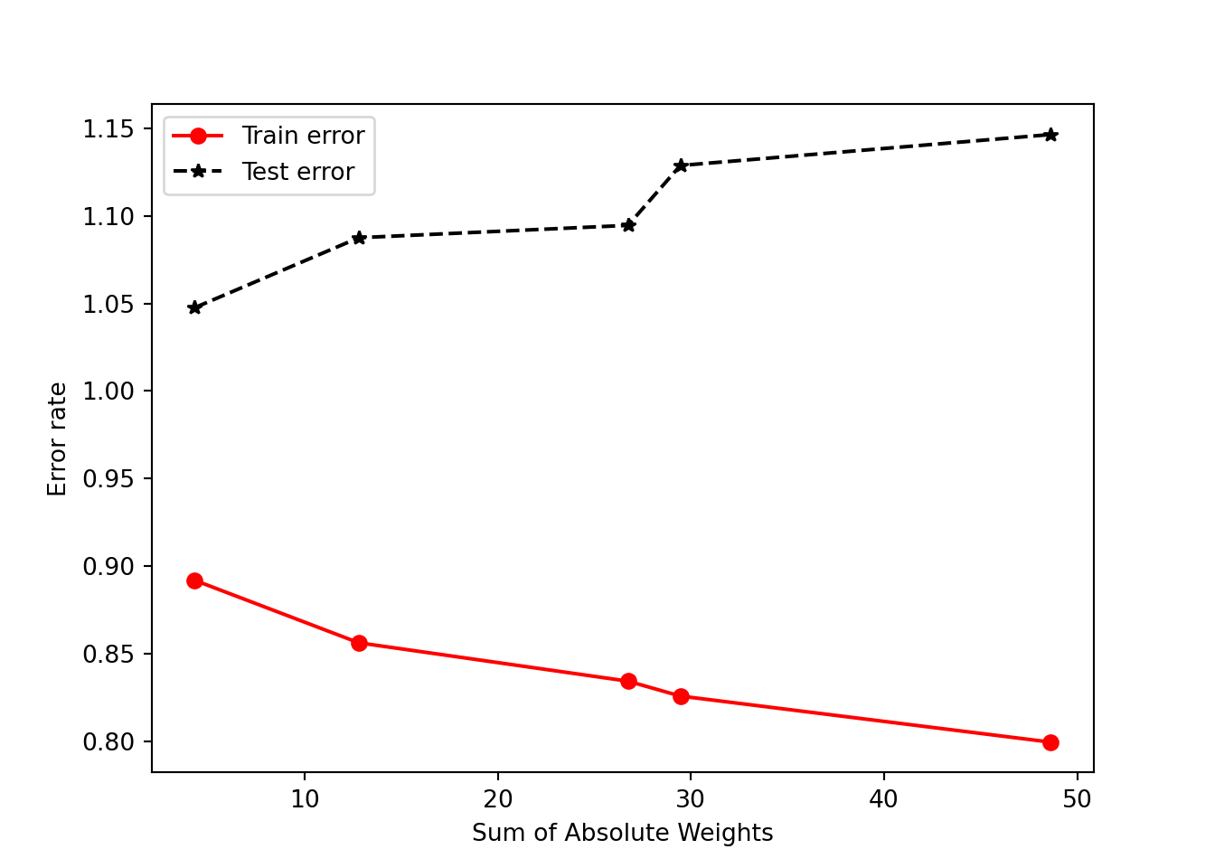
For postprocessing, we compute both the training and test errors of the models. We can also show the resulting model and the sum of the absolute weights of the regression coefficients, i.e., \(\sum_{j=0}^d |w_j|\), where \(d\) is the number of predictor attributes.
                                               Model  ...  Sum of Absolute Weights
0                                     -3.24 X + 1.08  ...                 4.322954
1                           -5.90 X + 5.92 X2 + 1.00  ...                12.817040
2               -6.22 X + -2.30 X2 + 17.14 X3 + 1.08  ...                26.744867
3      -7.16 X + 0.93 X2 + 8.39 X3 + 11.85 X4 + 1.12  ...                29.453660
4  -7.16 X + 4.50 X2 + 3.52 X3 + -6.55 X4 + 25.68...  ...                48.614927

[5 rows x 4 columns]
The results above show that the first model, which fits y against X only, has the largest training error, but smallest test error, whereas the fifth model, which fits y against X and other correlated attributes, has the smallest training error but largest test error. This is due to a phenomenon known as model overfitting, in which the low training error of the model does not reflect how well the model will perform on previously unseen test instances. From the plot shown above, observe that the disparity between the training and test errors becomes wider as the sum of absolute weights of the model (which represents the model complexity) increases. Thus, one should control the complexity of the regression model to avoid the model overfitting problem.
Ridge Regression
Ridge regression is a variant of MLR designed to fit a linear model to the dataset by minimizing the following regularized least-square loss function:
where \(\alpha\) is the hyperparameter for ridge regression. Note that the ridge regression model reduces to MLR when \(\alpha = 0\). By increasing the value of \(\alpha\), we can control the complexity of the model as will be shown in the example below.
In the example shown below, we fit a ridge regression model to the previously created training set with correlated attributes. We compare the results of the ridge regression model against those obtained using MLR.
from sklearn import linear_modelridge = linear_model.Ridge(alpha=0.4)ridge.fit(X_train5, y_train)
Ridge(alpha=0.4)
In a Jupyter environment, please rerun this cell to show the HTML representation or trust the notebook. On GitHub, the HTML representation is unable to render, please try loading this page with nbviewer.org.
                                                   Model  ...  Sum of Absolute Weights
0                                         -3.24 X + 1.08  ...                 4.322954
1                               -5.90 X + 5.92 X2 + 1.00  ...                12.817040
2                   -6.22 X + -2.30 X2 + 17.14 X3 + 1.08  ...                26.744867
3          -7.16 X + 0.93 X2 + 8.39 X3 + 11.85 X4 + 1.12  ...                29.453660
4      -7.16 X + 4.50 X2 + 3.52 X3 + -6.55 X4 + 25.68...  ...                48.614927
Ridge  -2.24 X + -0.43 X2 + -0.14 X3 + -0.10 X4 + 0.0...  ...                 3.765759

[6 rows x 4 columns]
By setting an appropriate value for the hyperparameter, �, we can control the sum of absolute weights, thus producing a test error that is quite comparable to that of MLR without the correlated attributes.
Lasso Regression
One of the limitations of ridge regression is that, although it was able to reduce the regression coefficients associated with the correlated attributes and reduce the effect of model overfitting, the resulting model is still not sparse. Another variation of MLR, called lasso regression, is designed to produce sparser models by imposing an \(l_1\) regularization on the regression coefficients as shown below:
The example code below shows the results of applying lasso regression to the previously used correlated dataset.
from sklearn import linear_modellasso = linear_model.Lasso(alpha=0.02)lasso.fit(X_train5, y_train)
Lasso(alpha=0.02)
In a Jupyter environment, please rerun this cell to show the HTML representation or trust the notebook. On GitHub, the HTML representation is unable to render, please try loading this page with nbviewer.org.
                                                   Model  ...  Sum of Absolute Weights
0                                         -3.24 X + 1.08  ...                 4.322954
1                               -5.90 X + 5.92 X2 + 1.00  ...                12.817040
2                   -6.22 X + -2.30 X2 + 17.14 X3 + 1.08  ...                26.744867
3          -7.16 X + 0.93 X2 + 8.39 X3 + 11.85 X4 + 1.12  ...                29.453660
4      -7.16 X + 4.50 X2 + 3.52 X3 + -6.55 X4 + 25.68...  ...                48.614927
Ridge  -2.24 X + -0.43 X2 + -0.14 X3 + -0.10 X4 + 0.0...  ...                 3.765759
Lasso  -2.90 X + 0.00 X2 + 0.00 X3 + 0.00 X4 + 0.00 X...  ...                 3.856242

[7 rows x 4 columns]
Observe that the lasso regression model sets the coefficients for the correlated attributes, X2, X3, X4, and X5 to exactly zero unlike the ridge regression model. As a result, its test error is significantly better than that for ridge regression.
Hyperparameter Selection via Cross-Validation
While both ridge and lasso regression methods can potentially alleviate the model overfitting problem, one of the challenges is how to select the appropriate hyperparameter value, \(\alpha\). In the examples shown below, we demonstrate examples of using a 5-fold cross-validation method to select the best hyperparameter of the model. More details about the model selection problem and cross-validation method are described in Chapter 3 of the book.
In the first sample code below, we vary the hyperparameter \(\alpha\) for ridge regression to a range between 0.2 and 1.0. Using the RidgeCV() function, we can train a model with 5-fold cross-validation and select the best hyperparameter value.
In a Jupyter environment, please rerun this cell to show the HTML representation or trust the notebook. On GitHub, the HTML representation is unable to render, please try loading this page with nbviewer.org.
In a Jupyter environment, please rerun this cell to show the HTML representation or trust the notebook. On GitHub, the HTML representation is unable to render, please try loading this page with nbviewer.org.
                                                     Model  ...  Sum of Absolute Weights
0                                           -3.24 X + 1.08  ...                 4.322954
1                                 -5.90 X + 5.92 X2 + 1.00  ...                12.817040
2                     -6.22 X + -2.30 X2 + 17.14 X3 + 1.08  ...                26.744867
3            -7.16 X + 0.93 X2 + 8.39 X3 + 11.85 X4 + 1.12  ...                29.453660
4        -7.16 X + 4.50 X2 + 3.52 X3 + -6.55 X4 + 25.68...  ...                48.614927
RidgeCV  -2.74 X + -0.16 X2 + 0.09 X3 + 0.01 X4 + 0.21 ...  ...                 4.112120
LassoCV  -3.07 X + 0.00 X2 + 0.00 X3 + 0.00 X4 + 0.00 X...  ...                 4.089598

[7 rows x 4 columns]
Summary
This section presents example Python code for fitting linear regression models to a dataset. We also illustrate the problem of model overfitting and shows two alternative methods, called ridge and lasso regression, that can help alleviate such problem. While the model overfitting problem shown here is illustrated in the context of correlated attributes, the problem is more general and may arise due to other factors such as noise and other exceptional values in the data.