# First run this
install.packages("pacman")Data Preprocessing in R
Goal
Practice basic R commands/methods for descriptive data analysis. If you are already familiar with some of the commands/methods, practice the ones new to you.
Note: copying and pasting early in learning will not produce the results you are looking for, and will catch up to you eventually.
Submission
Please submit .r, .rmd, or .qmd files ONLY.
Installing required packages
library(pacman)

p_load(DBI, # DBI databases
       dlookr,
       here, # Reproducible/ standard directories
       janitor,
       RMySQL, # Utilizing MySQL drivers
       tidymodels, # Tidyverse format modeling (e.g., lm())
       tidyverse, # Data wrangling, manipulation, visualization
       qqplotr)
Loading data
CSV files (.csv)
data <- read_csv(here("data", "x.csv"))

data |> glimpse()
Rows: 4 Columns: 3
── Column specification ────────────────────────────────────────────────────────
Delimiter: ","
chr (1): Name
dbl (2): ID, Age
ℹ Use `spec()` to retrieve the full column specification for this data.
ℹ Specify the column types or set `show_col_types = FALSE` to quiet this message.Rows: 4
Columns: 3
$ ID <dbl> 12345, 12346, 12347, 12348
$ Name <chr> "Amy", "Ana", "June", "May"
$ Age <dbl> 13, 14, 25, 21The |> is the Base R pipe as opposed to the magrittr pipe |>. The |> pipe can be utilized for most functions in R, while the |> pipe is more restricted towards the tidyverse.
Tab separated values (x.tsv)
data <- read_delim(here("data", "x.tsv"))

data |> glimpse()
Rows: 4 Columns: 3
── Column specification ────────────────────────────────────────────────────────
Delimiter: "\t"
chr (1): Name
dbl (2): ID, Age
ℹ Use `spec()` to retrieve the full column specification for this data.
ℹ Specify the column types or set `show_col_types = FALSE` to quiet this message.Rows: 4
Columns: 3
$ ID <dbl> 12345, 12346, 12347, 12348
$ Name <chr> "Amy", "Ana", "June", "May"
$ Age <dbl> 13, 14, NA, 21Importing data from MySQL database
First connect to a database in a MySQL database management system, then query tables in the database to obtain desired dataset.
drv <- dbDriver("MySQL") #obtain the driver for MySQL, drivers available for other DBMSGet a connection to my local mysql database etcsite_charaparser. If you don’t have a local database handy, you can skip this exercise and just get the idea on what it takes to connect to a db.
Using dplyr instead
install.packages("dbplyr") #install but don’t run library() on this dbplyr.Obtain a connection
con <- src_mysql("etcsite_charaparser", user = "termsuser", password = "termspassword", host = "localhost")Get an entire table as tbl
allwords <- tbl(con, "1_allwords")
allwords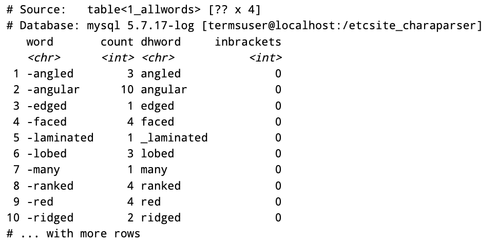
Next you can use methods in dplyr to select and filter if needed. DBI library allows you to use SQL query to select your data from db tables while dplyr library methods can be used when you don’t even know SQL language.
Importing extremely large dataset, consider data.table package’s fread(), or iotools package’s read.csv.raw().
Data Cleaning
Wide vs. long format
Read data in wide format
wide <- read_delim(here("data", "wide.txt"), delim = " ", skip = 1, col_names = c("Name", "Math", "English", "Degree_Year"))Rows: 3 Columns: 4
── Column specification ────────────────────────────────────────────────────────
Delimiter: " "
chr (2): Name, Degree_Year
dbl (2): Math, English
ℹ Use `spec()` to retrieve the full column specification for this data.
ℹ Specify the column types or set `show_col_types = FALSE` to quiet this message.# A tibble: 3 × 4
Name Math English Degree_Year
<chr> <dbl> <dbl> <chr>
1 Anna 86 90 Bio_2014
2 John 43 75 Math_2013
3 Cath 80 82 Bio_2012 The wide format uses the values (Math, English) of variable Subjects as variables.
The long format should have Name, Subject, and Grade as variables (i.e., columns).
long <- wide |>
  pivot_longer(cols = c(Math, English),
               names_to = "Subject",
               values_to = "Grade")
long
# A tibble: 6 × 4
Name Degree_Year Subject Grade
<chr> <chr> <chr> <dbl>
1 Anna Bio_2014 Math 86
2 Anna Bio_2014 English 90
3 John Math_2013 Math 43
4 John Math_2013 English 75
5 Cath Bio_2012 Math 80
6 Cath Bio_2012 English 82Long to wide, use spread()
wide <- long %>%
  pivot_wider(names_from = Subject, values_from = Grade)
wide
# A tibble: 3 × 4
Name Degree_Year Math English
<chr> <chr> <dbl> <dbl>
1 Anna Bio_2014 86 90
2 John Math_2013 43 75
3 Cath Bio_2012 80 82Split a column into multiple columns
Split Degree_Year to Degree and Year
clean <- long %>%
  separate(Degree_Year, c("Degree", "Year"), sep = "_")

clean
# A tibble: 6 × 5
Name Degree Year Subject Grade
<chr> <chr> <chr> <chr> <dbl>
1 Anna Bio 2014 Math 86
2 Anna Bio 2014 English 90
3 John Math 2013 Math 43
4 John Math 2013 English 75
5 Cath Bio 2012 Math 80
6 Cath Bio 2012 English 82Handling date/time and time zones
install.packages("lubridate")
library(lubridate)
Convert dates of variance formats into one format:
mixed.dates <- c(20140123, "2019-12-12", "2009/5/1",
 "measured on 2002-12-06", "2018-7/16")
clean.dates <- ymd(mixed.dates) #convert to year-month-day format
clean.dates
[1] "2014-01-23" "2019-12-12" "2009-05-01" "2002-12-06" "2018-07-16"Extract day, week, month, year info from dates:
data.frame(Dates = clean.dates, WeekDay = wday(clean.dates), nWeekDay = wday(clean.dates, label = TRUE), Year = year(clean.dates), Month = month(clean.dates, label = TRUE)) Dates WeekDay nWeekDay Year Month
1 2014-01-23 5 Thu 2014 Jan
2 2019-12-12 5 Thu 2019 Dec
3 2009-05-01 6 Fri 2009 May
4 2002-12-06 6 Fri 2002 Dec
5 2018-07-16 2 Mon 2018 JulTime zone:
date.time <- ymd_hms("20190203 03:00:03", tz="Asia/Shanghai")Convert to Phoenix, AZ time:
with_tz(date.time, tz="America/Phoenix")[1] "2019-02-02 12:00:03 MST"Change the timezone for a time:
force_tz(date.time, "Turkey")[1] "2019-02-03 03:00:03 +03"Check available time zones:
OlsonNames() [1] "Africa/Abidjan" "Africa/Accra"
[3] "Africa/Addis_Ababa" "Africa/Algiers"
[5] "Africa/Asmara" "Africa/Asmera"
[7] "Africa/Bamako" "Africa/Bangui"
[9] "Africa/Banjul" "Africa/Bissau"
[11] "Africa/Blantyre" "Africa/Brazzaville"
[13] "Africa/Bujumbura" "Africa/Cairo"
[15] "Africa/Casablanca" "Africa/Ceuta"
[17] "Africa/Conakry" "Africa/Dakar"
[19] "Africa/Dar_es_Salaam" "Africa/Djibouti"
[21] "Africa/Douala" "Africa/El_Aaiun"
[23] "Africa/Freetown" "Africa/Gaborone"
[25] "Africa/Harare" "Africa/Johannesburg"
[27] "Africa/Juba" "Africa/Kampala"
[29] "Africa/Khartoum" "Africa/Kigali"
[31] "Africa/Kinshasa" "Africa/Lagos"
[33] "Africa/Libreville" "Africa/Lome"
[35] "Africa/Luanda" "Africa/Lubumbashi"
[37] "Africa/Lusaka" "Africa/Malabo"
[39] "Africa/Maputo" "Africa/Maseru"
[41] "Africa/Mbabane" "Africa/Mogadishu"
[43] "Africa/Monrovia" "Africa/Nairobi"
[45] "Africa/Ndjamena" "Africa/Niamey"
[47] "Africa/Nouakchott" "Africa/Ouagadougou"
[49] "Africa/Porto-Novo" "Africa/Sao_Tome"
[51] "Africa/Timbuktu" "Africa/Tripoli"
[53] "Africa/Tunis" "Africa/Windhoek"
[55] "America/Adak" "America/Anchorage"
[57] "America/Anguilla" "America/Antigua"
[59] "America/Araguaina" "America/Argentina/Buenos_Aires"
[61] "America/Argentina/Catamarca" "America/Argentina/ComodRivadavia"
[63] "America/Argentina/Cordoba" "America/Argentina/Jujuy"
[65] "America/Argentina/La_Rioja" "America/Argentina/Mendoza"
[67] "America/Argentina/Rio_Gallegos" "America/Argentina/Salta"
[69] "America/Argentina/San_Juan" "America/Argentina/San_Luis"
[71] "America/Argentina/Tucuman" "America/Argentina/Ushuaia"
[73] "America/Aruba" "America/Asuncion"
[75] "America/Atikokan" "America/Atka"
[77] "America/Bahia" "America/Bahia_Banderas"
[79] "America/Barbados" "America/Belem"
[81] "America/Belize" "America/Blanc-Sablon"
[83] "America/Boa_Vista" "America/Bogota"
[85] "America/Boise" "America/Buenos_Aires"
[87] "America/Cambridge_Bay" "America/Campo_Grande"
[89] "America/Cancun" "America/Caracas"
[91] "America/Catamarca" "America/Cayenne"
[93] "America/Cayman" "America/Chicago"
[95] "America/Chihuahua" "America/Ciudad_Juarez"
[97] "America/Coral_Harbour" "America/Cordoba"
[99] "America/Costa_Rica" "America/Creston"
[101] "America/Cuiaba" "America/Curacao"
[103] "America/Danmarkshavn" "America/Dawson"
[105] "America/Dawson_Creek" "America/Denver"
[107] "America/Detroit" "America/Dominica"
[109] "America/Edmonton" "America/Eirunepe"
[111] "America/El_Salvador" "America/Ensenada"
[113] "America/Fort_Nelson" "America/Fort_Wayne"
[115] "America/Fortaleza" "America/Glace_Bay"
[117] "America/Godthab" "America/Goose_Bay"
[119] "America/Grand_Turk" "America/Grenada"
[121] "America/Guadeloupe" "America/Guatemala"
[123] "America/Guayaquil" "America/Guyana"
[125] "America/Halifax" "America/Havana"
[127] "America/Hermosillo" "America/Indiana/Indianapolis"
[129] "America/Indiana/Knox" "America/Indiana/Marengo"
[131] "America/Indiana/Petersburg" "America/Indiana/Tell_City"
[133] "America/Indiana/Vevay" "America/Indiana/Vincennes"
[135] "America/Indiana/Winamac" "America/Indianapolis"
[137] "America/Inuvik" "America/Iqaluit"
[139] "America/Jamaica" "America/Jujuy"
[141] "America/Juneau" "America/Kentucky/Louisville"
[143] "America/Kentucky/Monticello" "America/Knox_IN"
[145] "America/Kralendijk" "America/La_Paz"
[147] "America/Lima" "America/Los_Angeles"
[149] "America/Louisville" "America/Lower_Princes"
[151] "America/Maceio" "America/Managua"
[153] "America/Manaus" "America/Marigot"
[155] "America/Martinique" "America/Matamoros"
[157] "America/Mazatlan" "America/Mendoza"
[159] "America/Menominee" "America/Merida"
[161] "America/Metlakatla" "America/Mexico_City"
[163] "America/Miquelon" "America/Moncton"
[165] "America/Monterrey" "America/Montevideo"
[167] "America/Montreal" "America/Montserrat"
[169] "America/Nassau" "America/New_York"
[171] "America/Nipigon" "America/Nome"
[173] "America/Noronha" "America/North_Dakota/Beulah"
[175] "America/North_Dakota/Center" "America/North_Dakota/New_Salem"
[177] "America/Nuuk" "America/Ojinaga"
[179] "America/Panama" "America/Pangnirtung"
[181] "America/Paramaribo" "America/Phoenix"
[183] "America/Port_of_Spain" "America/Port-au-Prince"
[185] "America/Porto_Acre" "America/Porto_Velho"
[187] "America/Puerto_Rico" "America/Punta_Arenas"
[189] "America/Rainy_River" "America/Rankin_Inlet"
[191] "America/Recife" "America/Regina"
[193] "America/Resolute" "America/Rio_Branco"
[195] "America/Rosario" "America/Santa_Isabel"
[197] "America/Santarem" "America/Santiago"
[199] "America/Santo_Domingo" "America/Sao_Paulo"
[201] "America/Scoresbysund" "America/Shiprock"
[203] "America/Sitka" "America/St_Barthelemy"
[205] "America/St_Johns" "America/St_Kitts"
[207] "America/St_Lucia" "America/St_Thomas"
[209] "America/St_Vincent" "America/Swift_Current"
[211] "America/Tegucigalpa" "America/Thule"
[213] "America/Thunder_Bay" "America/Tijuana"
[215] "America/Toronto" "America/Tortola"
[217] "America/Vancouver" "America/Virgin"
[219] "America/Whitehorse" "America/Winnipeg"
[221] "America/Yakutat" "America/Yellowknife"
[223] "Antarctica/Casey" "Antarctica/Davis"
[225] "Antarctica/DumontDUrville" "Antarctica/Macquarie"
[227] "Antarctica/Mawson" "Antarctica/McMurdo"
[229] "Antarctica/Palmer" "Antarctica/Rothera"
[231] "Antarctica/South_Pole" "Antarctica/Syowa"
[233] "Antarctica/Troll" "Antarctica/Vostok"
[235] "Arctic/Longyearbyen" "Asia/Aden"
[237] "Asia/Almaty" "Asia/Amman"
[239] "Asia/Anadyr" "Asia/Aqtau"
[241] "Asia/Aqtobe" "Asia/Ashgabat"
[243] "Asia/Ashkhabad" "Asia/Atyrau"
[245] "Asia/Baghdad" "Asia/Bahrain"
[247] "Asia/Baku" "Asia/Bangkok"
[249] "Asia/Barnaul" "Asia/Beirut"
[251] "Asia/Bishkek" "Asia/Brunei"
[253] "Asia/Calcutta" "Asia/Chita"
[255] "Asia/Choibalsan" "Asia/Chongqing"
[257] "Asia/Chungking" "Asia/Colombo"
[259] "Asia/Dacca" "Asia/Damascus"
[261] "Asia/Dhaka" "Asia/Dili"
[263] "Asia/Dubai" "Asia/Dushanbe"
[265] "Asia/Famagusta" "Asia/Gaza"
[267] "Asia/Harbin" "Asia/Hebron"
[269] "Asia/Ho_Chi_Minh" "Asia/Hong_Kong"
[271] "Asia/Hovd" "Asia/Irkutsk"
[273] "Asia/Istanbul" "Asia/Jakarta"
[275] "Asia/Jayapura" "Asia/Jerusalem"
[277] "Asia/Kabul" "Asia/Kamchatka"
[279] "Asia/Karachi" "Asia/Kashgar"
[281] "Asia/Kathmandu" "Asia/Katmandu"
[283] "Asia/Khandyga" "Asia/Kolkata"
[285] "Asia/Krasnoyarsk" "Asia/Kuala_Lumpur"
[287] "Asia/Kuching" "Asia/Kuwait"
[289] "Asia/Macao" "Asia/Macau"
[291] "Asia/Magadan" "Asia/Makassar"
[293] "Asia/Manila" "Asia/Muscat"
[295] "Asia/Nicosia" "Asia/Novokuznetsk"
[297] "Asia/Novosibirsk" "Asia/Omsk"
[299] "Asia/Oral" "Asia/Phnom_Penh"
[301] "Asia/Pontianak" "Asia/Pyongyang"
[303] "Asia/Qatar" "Asia/Qostanay"
[305] "Asia/Qyzylorda" "Asia/Rangoon"
[307] "Asia/Riyadh" "Asia/Saigon"
[309] "Asia/Sakhalin" "Asia/Samarkand"
[311] "Asia/Seoul" "Asia/Shanghai"
[313] "Asia/Singapore" "Asia/Srednekolymsk"
[315] "Asia/Taipei" "Asia/Tashkent"
[317] "Asia/Tbilisi" "Asia/Tehran"
[319] "Asia/Tel_Aviv" "Asia/Thimbu"
[321] "Asia/Thimphu" "Asia/Tokyo"
[323] "Asia/Tomsk" "Asia/Ujung_Pandang"
[325] "Asia/Ulaanbaatar" "Asia/Ulan_Bator"
[327] "Asia/Urumqi" "Asia/Ust-Nera"
[329] "Asia/Vientiane" "Asia/Vladivostok"
[331] "Asia/Yakutsk" "Asia/Yangon"
[333] "Asia/Yekaterinburg" "Asia/Yerevan"
[335] "Atlantic/Azores" "Atlantic/Bermuda"
[337] "Atlantic/Canary" "Atlantic/Cape_Verde"
[339] "Atlantic/Faeroe" "Atlantic/Faroe"
[341] "Atlantic/Jan_Mayen" "Atlantic/Madeira"
[343] "Atlantic/Reykjavik" "Atlantic/South_Georgia"
[345] "Atlantic/St_Helena" "Atlantic/Stanley"
[347] "Australia/ACT" "Australia/Adelaide"
[349] "Australia/Brisbane" "Australia/Broken_Hill"
[351] "Australia/Canberra" "Australia/Currie"
[353] "Australia/Darwin" "Australia/Eucla"
[355] "Australia/Hobart" "Australia/LHI"
[357] "Australia/Lindeman" "Australia/Lord_Howe"
[359] "Australia/Melbourne" "Australia/North"
[361] "Australia/NSW" "Australia/Perth"
[363] "Australia/Queensland" "Australia/South"
[365] "Australia/Sydney" "Australia/Tasmania"
[367] "Australia/Victoria" "Australia/West"
[369] "Australia/Yancowinna" "Brazil/Acre"
[371] "Brazil/DeNoronha" "Brazil/East"
[373] "Brazil/West" "Canada/Atlantic"
[375] "Canada/Central" "Canada/Eastern"
[377] "Canada/Mountain" "Canada/Newfoundland"
[379] "Canada/Pacific" "Canada/Saskatchewan"
[381] "Canada/Yukon" "CET"
[383] "Chile/Continental" "Chile/EasterIsland"
[385] "CST6CDT" "Cuba"
[387] "EET" "Egypt"
[389] "Eire" "EST"
[391] "EST5EDT" "Etc/GMT"
[393] "Etc/GMT-0" "Etc/GMT-1"
[395] "Etc/GMT-10" "Etc/GMT-11"
[397] "Etc/GMT-12" "Etc/GMT-13"
[399] "Etc/GMT-14" "Etc/GMT-2"
[401] "Etc/GMT-3" "Etc/GMT-4"
[403] "Etc/GMT-5" "Etc/GMT-6"
[405] "Etc/GMT-7" "Etc/GMT-8"
[407] "Etc/GMT-9" "Etc/GMT+0"
[409] "Etc/GMT+1" "Etc/GMT+10"
[411] "Etc/GMT+11" "Etc/GMT+12"
[413] "Etc/GMT+2" "Etc/GMT+3"
[415] "Etc/GMT+4" "Etc/GMT+5"
[417] "Etc/GMT+6" "Etc/GMT+7"
[419] "Etc/GMT+8" "Etc/GMT+9"
[421] "Etc/GMT0" "Etc/Greenwich"
[423] "Etc/UCT" "Etc/Universal"
[425] "Etc/UTC" "Etc/Zulu"
[427] "Europe/Amsterdam" "Europe/Andorra"
[429] "Europe/Astrakhan" "Europe/Athens"
[431] "Europe/Belfast" "Europe/Belgrade"
[433] "Europe/Berlin" "Europe/Bratislava"
[435] "Europe/Brussels" "Europe/Bucharest"
[437] "Europe/Budapest" "Europe/Busingen"
[439] "Europe/Chisinau" "Europe/Copenhagen"
[441] "Europe/Dublin" "Europe/Gibraltar"
[443] "Europe/Guernsey" "Europe/Helsinki"
[445] "Europe/Isle_of_Man" "Europe/Istanbul"
[447] "Europe/Jersey" "Europe/Kaliningrad"
[449] "Europe/Kiev" "Europe/Kirov"
[451] "Europe/Kyiv" "Europe/Lisbon"
[453] "Europe/Ljubljana" "Europe/London"
[455] "Europe/Luxembourg" "Europe/Madrid"
[457] "Europe/Malta" "Europe/Mariehamn"
[459] "Europe/Minsk" "Europe/Monaco"
[461] "Europe/Moscow" "Europe/Nicosia"
[463] "Europe/Oslo" "Europe/Paris"
[465] "Europe/Podgorica" "Europe/Prague"
[467] "Europe/Riga" "Europe/Rome"
[469] "Europe/Samara" "Europe/San_Marino"
[471] "Europe/Sarajevo" "Europe/Saratov"
[473] "Europe/Simferopol" "Europe/Skopje"
[475] "Europe/Sofia" "Europe/Stockholm"
[477] "Europe/Tallinn" "Europe/Tirane"
[479] "Europe/Tiraspol" "Europe/Ulyanovsk"
[481] "Europe/Uzhgorod" "Europe/Vaduz"
[483] "Europe/Vatican" "Europe/Vienna"
[485] "Europe/Vilnius" "Europe/Volgograd"
[487] "Europe/Warsaw" "Europe/Zagreb"
[489] "Europe/Zaporozhye" "Europe/Zurich"
[491] "Factory" "GB"
[493] "GB-Eire" "GMT"
[495] "GMT-0" "GMT+0"
[497] "GMT0" "Greenwich"
[499] "Hongkong" "HST"
[501] "Iceland" "Indian/Antananarivo"
[503] "Indian/Chagos" "Indian/Christmas"
[505] "Indian/Cocos" "Indian/Comoro"
[507] "Indian/Kerguelen" "Indian/Mahe"
[509] "Indian/Maldives" "Indian/Mauritius"
[511] "Indian/Mayotte" "Indian/Reunion"
[513] "Iran" "Israel"
[515] "Jamaica" "Japan"
[517] "Kwajalein" "Libya"
[519] "MET" "Mexico/BajaNorte"
[521] "Mexico/BajaSur" "Mexico/General"
[523] "MST" "MST7MDT"
[525] "Navajo" "NZ"
[527] "NZ-CHAT" "Pacific/Apia"
[529] "Pacific/Auckland" "Pacific/Bougainville"
[531] "Pacific/Chatham" "Pacific/Chuuk"
[533] "Pacific/Easter" "Pacific/Efate"
[535] "Pacific/Enderbury" "Pacific/Fakaofo"
[537] "Pacific/Fiji" "Pacific/Funafuti"
[539] "Pacific/Galapagos" "Pacific/Gambier"
[541] "Pacific/Guadalcanal" "Pacific/Guam"
[543] "Pacific/Honolulu" "Pacific/Johnston"
[545] "Pacific/Kanton" "Pacific/Kiritimati"
[547] "Pacific/Kosrae" "Pacific/Kwajalein"
[549] "Pacific/Majuro" "Pacific/Marquesas"
[551] "Pacific/Midway" "Pacific/Nauru"
[553] "Pacific/Niue" "Pacific/Norfolk"
[555] "Pacific/Noumea" "Pacific/Pago_Pago"
[557] "Pacific/Palau" "Pacific/Pitcairn"
[559] "Pacific/Pohnpei" "Pacific/Ponape"
[561] "Pacific/Port_Moresby" "Pacific/Rarotonga"
[563] "Pacific/Saipan" "Pacific/Samoa"
[565] "Pacific/Tahiti" "Pacific/Tarawa"
[567] "Pacific/Tongatapu" "Pacific/Truk"
[569] "Pacific/Wake" "Pacific/Wallis"
[571] "Pacific/Yap" "Poland"
[573] "Portugal" "PRC"
[575] "PST8PDT" "ROC"
[577] "ROK" "Singapore"
[579] "Turkey" "UCT"
[581] "Universal" "US/Alaska"
[583] "US/Aleutian" "US/Arizona"
[585] "US/Central" "US/East-Indiana"
[587] "US/Eastern" "US/Hawaii"
[589] "US/Indiana-Starke" "US/Michigan"
[591] "US/Mountain" "US/Pacific"
[593] "US/Samoa" "UTC"
[595] "W-SU" "WET"
[597] "Zulu"
attr(,"Version")
[1] "2023c"String Processing
Common needs: stringr package
Advanced needs: stringi package
The following code shows the use of functions provided by stringr package to put column names back to a dataset fetched from http://archive.ics.uci.edu/ml/machine-learning-databases/audiology/
library(dplyr)
library(stringr)
library(readr)
Fetch data from a URL, form the URL using string functions:
uci.repo <-"http://archive.ics.uci.edu/ml/machine-learning-databases/"

dataset <- "audiology/audiology.standardized"str_c: string concatenation:
dataF <- str_c(uci.repo, dataset, ".data")
namesF <- str_c(uci.repo, dataset, ".names")
dataF
[1] "http://archive.ics.uci.edu/ml/machine-learning-databases/audiology/audiology.standardized.data"Read the data file:
data <- read_csv(url(dataF), col_names = FALSE, na="?")Rows: 200 Columns: 71
── Column specification ────────────────────────────────────────────────────────
Delimiter: ","
chr (11): X2, X4, X5, X6, X8, X59, X60, X64, X66, X70, X71
lgl (60): X1, X3, X7, X9, X10, X11, X12, X13, X14, X15, X16, X17, X18, X19, ...
ℹ Use `spec()` to retrieve the full column specification for this data.
ℹ Specify the column types or set `show_col_types = FALSE` to quiet this message.dim(data)[1] 200 71Read the name file line by line, put the lines in a vector:
lines <- read_lines(url(namesF))

lines |> head()
[1] "WARNING: This database should be credited to the original owner whenever"
[2] " used for any publication whatsoever."
[3] ""
[4] "1. Title: Standardized Audiology Database "
[5] ""
[6] "2. Sources:" Examine the content of lines and see the column names start on line 67, ends on line 135. Then, get column name lines and clean up to get column names:
names <- lines[67:135]
names
[1] " age_gt_60:\t\t f, t."
[2] " air():\t\t mild,moderate,severe,normal,profound."
[3] " airBoneGap:\t\t f, t."
[4] " ar_c():\t\t normal,elevated,absent."
[5] " ar_u():\t\t normal,absent,elevated."
[6] " bone():\t\t mild,moderate,normal,unmeasured."
[7] " boneAbnormal:\t f, t."
[8] " bser():\t\t normal,degraded."
[9] " history_buzzing:\t f, t."
[10] " history_dizziness:\t f, t."
[11] " history_fluctuating:\t f, t."
[12] " history_fullness:\t f, t."
[13] " history_heredity:\t f, t."
[14] " history_nausea:\t f, t."
[15] " history_noise:\t f, t."
[16] " history_recruitment:\t f, t."
[17] " history_ringing:\t f, t."
[18] " history_roaring:\t f, t."
[19] " history_vomiting:\t f, t."
[20] " late_wave_poor:\t f, t."
[21] " m_at_2k:\t\t f, t."
[22] " m_cond_lt_1k:\t f, t."
[23] " m_gt_1k:\t\t f, t."
[24] " m_m_gt_2k:\t\t f, t."
[25] " m_m_sn:\t\t f, t."
[26] " m_m_sn_gt_1k:\t f, t."
[27] " m_m_sn_gt_2k:\t f, t."
[28] " m_m_sn_gt_500:\t f, t."
[29] " m_p_sn_gt_2k:\t f, t."
[30] " m_s_gt_500:\t\t f, t."
[31] " m_s_sn:\t\t f, t."
[32] " m_s_sn_gt_1k:\t f, t."
[33] " m_s_sn_gt_2k:\t f, t."
[34] " m_s_sn_gt_3k:\t f, t."
[35] " m_s_sn_gt_4k:\t f, t."
[36] " m_sn_2_3k:\t\t f, t."
[37] " m_sn_gt_1k:\t\t f, t."
[38] " m_sn_gt_2k:\t\t f, t."
[39] " m_sn_gt_3k:\t\t f, t."
[40] " m_sn_gt_4k:\t\t f, t."
[41] " m_sn_gt_500:\t\t f, t."
[42] " m_sn_gt_6k:\t\t f, t."
[43] " m_sn_lt_1k:\t\t f, t. "
[44] " m_sn_lt_2k:\t\t f, t."
[45] " m_sn_lt_3k:\t\t f, t."
[46] " middle_wave_poor:\t f, t."
[47] " mod_gt_4k:\t\t f, t."
[48] " mod_mixed:\t\t f, t."
[49] " mod_s_mixed:\t\t f, t."
[50] " mod_s_sn_gt_500:\t f, t."
[51] " mod_sn:\t\t f, t."
[52] " mod_sn_gt_1k:\t f, t."
[53] " mod_sn_gt_2k:\t f, t."
[54] " mod_sn_gt_3k:\t f, t."
[55] " mod_sn_gt_4k:\t f, t."
[56] " mod_sn_gt_500:\t f, t."
[57] " notch_4k:\t\t f, t."
[58] " notch_at_4k:\t\t f, t."
[59] " o_ar_c():\t\t normal,elevated,absent."
[60] " o_ar_u():\t\t normal,absent,elevated."
[61] " s_sn_gt_1k:\t\t f, t."
[62] " s_sn_gt_2k:\t\t f, t."
[63] " s_sn_gt_4k:\t\t f, t."
[64] " speech():\t\t normal,good,very_good,very_poor,poor,unmeasured."
[65] " static_normal:\t f, t."
[66] " tymp():\t\t a,as,b,ad,c."
[67] " viith_nerve_signs: f, t."
[68] " wave_V_delayed:\t f, t."
[69] " waveform_ItoV_prolonged: f, t." Observe: a name line consists two parts, name: valid values. The part before : is the name.
names <- str_split_fixed(names, ":", 2) #split on regular expression pattern ":", this function returns a matrix
names
[,1]
[1,] " age_gt_60"
[2,] " air()"
[3,] " airBoneGap"
[4,] " ar_c()"
[5,] " ar_u()"
[6,] " bone()"
[7,] " boneAbnormal"
[8,] " bser()"
[9,] " history_buzzing"
[10,] " history_dizziness"
[11,] " history_fluctuating"
[12,] " history_fullness"
[13,] " history_heredity"
[14,] " history_nausea"
[15,] " history_noise"
[16,] " history_recruitment"
[17,] " history_ringing"
[18,] " history_roaring"
[19,] " history_vomiting"
[20,] " late_wave_poor"
[21,] " m_at_2k"
[22,] " m_cond_lt_1k"
[23,] " m_gt_1k"
[24,] " m_m_gt_2k"
[25,] " m_m_sn"
[26,] " m_m_sn_gt_1k"
[27,] " m_m_sn_gt_2k"
[28,] " m_m_sn_gt_500"
[29,] " m_p_sn_gt_2k"
[30,] " m_s_gt_500"
[31,] " m_s_sn"
[32,] " m_s_sn_gt_1k"
[33,] " m_s_sn_gt_2k"
[34,] " m_s_sn_gt_3k"
[35,] " m_s_sn_gt_4k"
[36,] " m_sn_2_3k"
[37,] " m_sn_gt_1k"
[38,] " m_sn_gt_2k"
[39,] " m_sn_gt_3k"
[40,] " m_sn_gt_4k"
[41,] " m_sn_gt_500"
[42,] " m_sn_gt_6k"
[43,] " m_sn_lt_1k"
[44,] " m_sn_lt_2k"
[45,] " m_sn_lt_3k"
[46,] " middle_wave_poor"
[47,] " mod_gt_4k"
[48,] " mod_mixed"
[49,] " mod_s_mixed"
[50,] " mod_s_sn_gt_500"
[51,] " mod_sn"
[52,] " mod_sn_gt_1k"
[53,] " mod_sn_gt_2k"
[54,] " mod_sn_gt_3k"
[55,] " mod_sn_gt_4k"
[56,] " mod_sn_gt_500"
[57,] " notch_4k"
[58,] " notch_at_4k"
[59,] " o_ar_c()"
[60,] " o_ar_u()"
[61,] " s_sn_gt_1k"
[62,] " s_sn_gt_2k"
[63,] " s_sn_gt_4k"
[64,] " speech()"
[65,] " static_normal"
[66,] " tymp()"
[67,] " viith_nerve_signs"
[68,] " wave_V_delayed"
[69,] " waveform_ItoV_prolonged"
[,2]
[1,] "\t\t f, t."
[2,] "\t\t mild,moderate,severe,normal,profound."
[3,] "\t\t f, t."
[4,] "\t\t normal,elevated,absent."
[5,] "\t\t normal,absent,elevated."
[6,] "\t\t mild,moderate,normal,unmeasured."
[7,] "\t f, t."
[8,] "\t\t normal,degraded."
[9,] "\t f, t."
[10,] "\t f, t."
[11,] "\t f, t."
[12,] "\t f, t."
[13,] "\t f, t."
[14,] "\t f, t."
[15,] "\t f, t."
[16,] "\t f, t."
[17,] "\t f, t."
[18,] "\t f, t."
[19,] "\t f, t."
[20,] "\t f, t."
[21,] "\t\t f, t."
[22,] "\t f, t."
[23,] "\t\t f, t."
[24,] "\t\t f, t."
[25,] "\t\t f, t."
[26,] "\t f, t."
[27,] "\t f, t."
[28,] "\t f, t."
[29,] "\t f, t."
[30,] "\t\t f, t."
[31,] "\t\t f, t."
[32,] "\t f, t."
[33,] "\t f, t."
[34,] "\t f, t."
[35,] "\t f, t."
[36,] "\t\t f, t."
[37,] "\t\t f, t."
[38,] "\t\t f, t."
[39,] "\t\t f, t."
[40,] "\t\t f, t."
[41,] "\t\t f, t."
[42,] "\t\t f, t."
[43,] "\t\t f, t. "
[44,] "\t\t f, t."
[45,] "\t\t f, t."
[46,] "\t f, t."
[47,] "\t\t f, t."
[48,] "\t\t f, t."
[49,] "\t\t f, t."
[50,] "\t f, t."
[51,] "\t\t f, t."
[52,] "\t f, t."
[53,] "\t f, t."
[54,] "\t f, t."
[55,] "\t f, t."
[56,] "\t f, t."
[57,] "\t\t f, t."
[58,] "\t\t f, t."
[59,] "\t\t normal,elevated,absent."
[60,] "\t\t normal,absent,elevated."
[61,] "\t\t f, t."
[62,] "\t\t f, t."
[63,] "\t\t f, t."
[64,] "\t\t normal,good,very_good,very_poor,poor,unmeasured."
[65,] "\t f, t."
[66,] "\t\t a,as,b,ad,c."
[67,] " f, t."
[68,] "\t f, t."
[69,] " f, t." Take the first column, which contains names:
names <- names[,1]
names
[1] " age_gt_60" " air()"
[3] " airBoneGap" " ar_c()"
[5] " ar_u()" " bone()"
[7] " boneAbnormal" " bser()"
[9] " history_buzzing" " history_dizziness"
[11] " history_fluctuating" " history_fullness"
[13] " history_heredity" " history_nausea"
[15] " history_noise" " history_recruitment"
[17] " history_ringing" " history_roaring"
[19] " history_vomiting" " late_wave_poor"
[21] " m_at_2k" " m_cond_lt_1k"
[23] " m_gt_1k" " m_m_gt_2k"
[25] " m_m_sn" " m_m_sn_gt_1k"
[27] " m_m_sn_gt_2k" " m_m_sn_gt_500"
[29] " m_p_sn_gt_2k" " m_s_gt_500"
[31] " m_s_sn" " m_s_sn_gt_1k"
[33] " m_s_sn_gt_2k" " m_s_sn_gt_3k"
[35] " m_s_sn_gt_4k" " m_sn_2_3k"
[37] " m_sn_gt_1k" " m_sn_gt_2k"
[39] " m_sn_gt_3k" " m_sn_gt_4k"
[41] " m_sn_gt_500" " m_sn_gt_6k"
[43] " m_sn_lt_1k" " m_sn_lt_2k"
[45] " m_sn_lt_3k" " middle_wave_poor"
[47] " mod_gt_4k" " mod_mixed"
[49] " mod_s_mixed" " mod_s_sn_gt_500"
[51] " mod_sn" " mod_sn_gt_1k"
[53] " mod_sn_gt_2k" " mod_sn_gt_3k"
[55] " mod_sn_gt_4k" " mod_sn_gt_500"
[57] " notch_4k" " notch_at_4k"
[59] " o_ar_c()" " o_ar_u()"
[61] " s_sn_gt_1k" " s_sn_gt_2k"
[63] " s_sn_gt_4k" " speech()"
[65] " static_normal" " tymp()"
[67] " viith_nerve_signs" " wave_V_delayed"
[69] " waveform_ItoV_prolonged"Now clean up the names: trim spaces, remove ():
names <-str_trim(names) |> str_replace_all("\\(|\\)", "") # we use a pipe, and another reg exp "\\(|\\)", \\ is the escape.
names
[1] "age_gt_60" "air"
[3] "airBoneGap" "ar_c"
[5] "ar_u" "bone"
[7] "boneAbnormal" "bser"
[9] "history_buzzing" "history_dizziness"
[11] "history_fluctuating" "history_fullness"
[13] "history_heredity" "history_nausea"
[15] "history_noise" "history_recruitment"
[17] "history_ringing" "history_roaring"
[19] "history_vomiting" "late_wave_poor"
[21] "m_at_2k" "m_cond_lt_1k"
[23] "m_gt_1k" "m_m_gt_2k"
[25] "m_m_sn" "m_m_sn_gt_1k"
[27] "m_m_sn_gt_2k" "m_m_sn_gt_500"
[29] "m_p_sn_gt_2k" "m_s_gt_500"
[31] "m_s_sn" "m_s_sn_gt_1k"
[33] "m_s_sn_gt_2k" "m_s_sn_gt_3k"
[35] "m_s_sn_gt_4k" "m_sn_2_3k"
[37] "m_sn_gt_1k" "m_sn_gt_2k"
[39] "m_sn_gt_3k" "m_sn_gt_4k"
[41] "m_sn_gt_500" "m_sn_gt_6k"
[43] "m_sn_lt_1k" "m_sn_lt_2k"
[45] "m_sn_lt_3k" "middle_wave_poor"
[47] "mod_gt_4k" "mod_mixed"
[49] "mod_s_mixed" "mod_s_sn_gt_500"
[51] "mod_sn" "mod_sn_gt_1k"
[53] "mod_sn_gt_2k" "mod_sn_gt_3k"
[55] "mod_sn_gt_4k" "mod_sn_gt_500"
[57] "notch_4k" "notch_at_4k"
[59] "o_ar_c" "o_ar_u"
[61] "s_sn_gt_1k" "s_sn_gt_2k"
[63] "s_sn_gt_4k" "speech"
[65] "static_normal" "tymp"
[67] "viith_nerve_signs" "wave_V_delayed"
[69] "waveform_ItoV_prolonged"Finally, put the columns to the data:
Note: data has 71 rows but we only has 69 names. The last two columns in data are identifier and class labels. So we will put the 69 names to the first 69 columns.
colnames(data)[1:69] <- names
data
# A tibble: 200 × 71
age_gt_60 air airBoneGap ar_c ar_u bone boneAbnormal bser
<lgl> <chr> <lgl> <chr> <chr> <chr> <lgl> <chr>
1 FALSE mild FALSE normal normal <NA> TRUE <NA>
2 FALSE moderate FALSE normal normal <NA> TRUE <NA>
3 TRUE mild TRUE <NA> absent mild TRUE <NA>
4 TRUE mild TRUE <NA> absent mild FALSE <NA>
5 TRUE mild FALSE normal normal mild TRUE <NA>
6 TRUE mild FALSE normal normal mild TRUE <NA>
7 FALSE mild FALSE normal normal mild TRUE <NA>
8 FALSE mild FALSE normal normal mild TRUE <NA>
9 FALSE severe FALSE <NA> <NA> <NA> TRUE <NA>
10 TRUE mild FALSE elevated absent mild TRUE <NA>
# ℹ 190 more rows
# ℹ 63 more variables: history_buzzing <lgl>, history_dizziness <lgl>,
# history_fluctuating <lgl>, history_fullness <lgl>, history_heredity <lgl>,
# history_nausea <lgl>, history_noise <lgl>, history_recruitment <lgl>,
# history_ringing <lgl>, history_roaring <lgl>, history_vomiting <lgl>,
# late_wave_poor <lgl>, m_at_2k <lgl>, m_cond_lt_1k <lgl>, m_gt_1k <lgl>,
# m_m_gt_2k <lgl>, m_m_sn <lgl>, m_m_sn_gt_1k <lgl>, m_m_sn_gt_2k <lgl>, …Rename the last two columns:
colnames(data)[70:71] <- c("id", "class")
data
# A tibble: 200 × 71
age_gt_60 air airBoneGap ar_c ar_u bone boneAbnormal bser
<lgl> <chr> <lgl> <chr> <chr> <chr> <lgl> <chr>
1 FALSE mild FALSE normal normal <NA> TRUE <NA>
2 FALSE moderate FALSE normal normal <NA> TRUE <NA>
3 TRUE mild TRUE <NA> absent mild TRUE <NA>
4 TRUE mild TRUE <NA> absent mild FALSE <NA>
5 TRUE mild FALSE normal normal mild TRUE <NA>
6 TRUE mild FALSE normal normal mild TRUE <NA>
7 FALSE mild FALSE normal normal mild TRUE <NA>
8 FALSE mild FALSE normal normal mild TRUE <NA>
9 FALSE severe FALSE <NA> <NA> <NA> TRUE <NA>
10 TRUE mild FALSE elevated absent mild TRUE <NA>
# ℹ 190 more rows
# ℹ 63 more variables: history_buzzing <lgl>, history_dizziness <lgl>,
# history_fluctuating <lgl>, history_fullness <lgl>, history_heredity <lgl>,
# history_nausea <lgl>, history_noise <lgl>, history_recruitment <lgl>,
# history_ringing <lgl>, history_roaring <lgl>, history_vomiting <lgl>,
# late_wave_poor <lgl>, m_at_2k <lgl>, m_cond_lt_1k <lgl>, m_gt_1k <lgl>,
# m_m_gt_2k <lgl>, m_m_sn <lgl>, m_m_sn_gt_1k <lgl>, m_m_sn_gt_2k <lgl>, …DONE!
Dealing with unknown values
Remove observations or columns with many NAs:
library(dplyr)

missing.value.rows <- data |>
  filter(!complete.cases(data))
missing.value.rows
# A tibble: 196 × 71
age_gt_60 air airBoneGap ar_c ar_u bone boneAbnormal bser
<lgl> <chr> <lgl> <chr> <chr> <chr> <lgl> <chr>
1 FALSE mild FALSE normal normal <NA> TRUE <NA>
2 FALSE moderate FALSE normal normal <NA> TRUE <NA>
3 TRUE mild TRUE <NA> absent mild TRUE <NA>
4 TRUE mild TRUE <NA> absent mild FALSE <NA>
5 TRUE mild FALSE normal normal mild TRUE <NA>
6 TRUE mild FALSE normal normal mild TRUE <NA>
7 FALSE mild FALSE normal normal mild TRUE <NA>
8 FALSE mild FALSE normal normal mild TRUE <NA>
9 FALSE severe FALSE <NA> <NA> <NA> TRUE <NA>
10 TRUE mild FALSE elevated absent mild TRUE <NA>
# ℹ 186 more rows
# ℹ 63 more variables: history_buzzing <lgl>, history_dizziness <lgl>,
# history_fluctuating <lgl>, history_fullness <lgl>, history_heredity <lgl>,
# history_nausea <lgl>, history_noise <lgl>, history_recruitment <lgl>,
# history_ringing <lgl>, history_roaring <lgl>, history_vomiting <lgl>,
# late_wave_poor <lgl>, m_at_2k <lgl>, m_cond_lt_1k <lgl>, m_gt_1k <lgl>,
# m_m_gt_2k <lgl>, m_m_sn <lgl>, m_m_sn_gt_1k <lgl>, m_m_sn_gt_2k <lgl>, …196 out of 200 rows contain an NA!
How many NAs in each row? Apply a temporary function to the rows (“1”, if to columns use “2”) of data. This function counts the number of NAs in a row. If is.na(x) is TRUE (equivalent to 1), the sum of the booleans is then the count.
data <- data %>%
  mutate(na_count = rowSums(is.na(data)))
data
# A tibble: 200 × 72
age_gt_60 air airBoneGap ar_c ar_u bone boneAbnormal bser
<lgl> <chr> <lgl> <chr> <chr> <chr> <lgl> <chr>
1 FALSE mild FALSE normal normal <NA> TRUE <NA>
2 FALSE moderate FALSE normal normal <NA> TRUE <NA>
3 TRUE mild TRUE <NA> absent mild TRUE <NA>
4 TRUE mild TRUE <NA> absent mild FALSE <NA>
5 TRUE mild FALSE normal normal mild TRUE <NA>
6 TRUE mild FALSE normal normal mild TRUE <NA>
7 FALSE mild FALSE normal normal mild TRUE <NA>
8 FALSE mild FALSE normal normal mild TRUE <NA>
9 FALSE severe FALSE <NA> <NA> <NA> TRUE <NA>
10 TRUE mild FALSE elevated absent mild TRUE <NA>
# ℹ 190 more rows
# ℹ 64 more variables: history_buzzing <lgl>, history_dizziness <lgl>,
# history_fluctuating <lgl>, history_fullness <lgl>, history_heredity <lgl>,
# history_nausea <lgl>, history_noise <lgl>, history_recruitment <lgl>,
# history_ringing <lgl>, history_roaring <lgl>, history_vomiting <lgl>,
# late_wave_poor <lgl>, m_at_2k <lgl>, m_cond_lt_1k <lgl>, m_gt_1k <lgl>,
# m_m_gt_2k <lgl>, m_m_sn <lgl>, m_m_sn_gt_1k <lgl>, m_m_sn_gt_2k <lgl>, …Maximum missing values in a row is 7, out of 69 dimensions, so they are not too bad.
Examine columns: how many NAs in each variable/column?
data |>
  summarize(across(everything(), ~sum(is.na(.)), .names = "na_{.col}")) %>%
  pivot_longer(everything(), names_to = "column_name", values_to = "na_count") %>%
  arrange(na_count)
# A tibble: 72 × 2
column_name na_count
<chr> <int>
1 na_age_gt_60 0
2 na_air 0
3 na_airBoneGap 0
4 na_boneAbnormal 0
5 na_history_buzzing 0
6 na_history_dizziness 0
7 na_history_fluctuating 0
8 na_history_fullness 0
9 na_history_heredity 0
10 na_history_nausea 0
# ℹ 62 more rowsbser variable has 196 NAs. If this variable is considered not useful, given some domain knowledge, we can remove it from the data. From View, I can see bser is the 8th column:
data.bser.removed <- data %>%
  select(-8) %>%
  summarise(across(everything(), ~sum(is.na(.)), .names = "na_{.col}"))
data.bser.removed
# A tibble: 1 × 71
na_age_gt_60 na_air na_airBoneGap na_ar_c na_ar_u na_bone na_boneAbnormal
<int> <int> <int> <int> <int> <int> <int>
1 0 0 0 4 3 75 0
# ℹ 64 more variables: na_history_buzzing <int>, na_history_dizziness <int>,
# na_history_fluctuating <int>, na_history_fullness <int>,
# na_history_heredity <int>, na_history_nausea <int>, na_history_noise <int>,
# na_history_recruitment <int>, na_history_ringing <int>,
# na_history_roaring <int>, na_history_vomiting <int>,
# na_late_wave_poor <int>, na_m_at_2k <int>, na_m_cond_lt_1k <int>,
# na_m_gt_1k <int>, na_m_m_gt_2k <int>, na_m_m_sn <int>, …matches function can also help you find the index of a colname given its name:
data <- data %>%
  select(-matches("bser"))
Mistaken characters
Because R decides the data type based on what is given, sometimes, R’s decision may not be what you meant. In the example below, because of a missing value ?, R makes all other values in a vector ‘character’. Parse_integer can be used to fix this problem.
mistaken <- c(2, 3, 4, "?")
class(mistaken)
[1] "character"fixed <- parse_integer(mistaken, na = '?')
fixed[1] 2 3 4 NAclass(fixed)[1] "integer"Filling unknowns with most frequent values
Always take cautions when you modify the original data.
!!!Modifications must be well documented (so others can repeat your analysis) and well justified!!!
install.packages("DMwR2")
library(DMwR2)
data(algae, package = "DMwR2")
algae[48,]
Registered S3 method overwritten by 'quantmod':
method from
as.zoo.data.frame zoo # A tibble: 1 × 18
season size speed mxPH mnO2 Cl NO3 NH4 oPO4 PO4 Chla a1 a2
<fct> <fct> <fct> <dbl> <dbl> <dbl> <dbl> <dbl> <dbl> <dbl> <dbl> <dbl> <dbl>
1 winter small low NA 12.6 9 0.23 10 5 6 1.1 35.5 0
# ℹ 5 more variables: a3 <dbl>, a4 <dbl>, a5 <dbl>, a6 <dbl>, a7 <dbl>mxPH is unknown. Shall we fill in with mean, median or something else?
# plot a QQ plot of mxPH
install.packages("car")
library(car)
ggplot(algae, aes(sample = mxPH)) +
  geom_qq_band() +
  stat_qq_point() +
    stat_qq_line(color = "red", method = "identity", intercept = -2, slope = 1) +
  ggtitle("Normal QQ plot of mxPH")
Loading required package: carData
Attaching package: 'car'The following object is masked from 'package:purrr':
someThe following object is masked from 'package:dplyr':
recodeWarning in stat_qq_line(color = "red", method = "identity", intercept = -2, :
Ignoring unknown parameters: `method`, `intercept`, and `slope`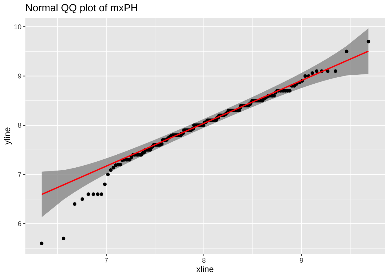
The straight line fits the data pretty well so mxPH is normal, use mean to fill the unknown.
algae <- algae |>
  mutate(mxPH = ifelse(row_number() == 48, mean(mxPH, na.rm = TRUE), mxPH))
algae
# A tibble: 200 × 18
season size speed mxPH mnO2 Cl NO3 NH4 oPO4 PO4 Chla a1
<fct> <fct> <fct> <dbl> <dbl> <dbl> <dbl> <dbl> <dbl> <dbl> <dbl> <dbl>
1 winter small medium 8 9.8 60.8 6.24 578 105 170 50 0
2 spring small medium 8.35 8 57.8 1.29 370 429. 559. 1.3 1.4
3 autumn small medium 8.1 11.4 40.0 5.33 347. 126. 187. 15.6 3.3
4 spring small medium 8.07 4.8 77.4 2.30 98.2 61.2 139. 1.4 3.1
5 autumn small medium 8.06 9 55.4 10.4 234. 58.2 97.6 10.5 9.2
6 winter small high 8.25 13.1 65.8 9.25 430 18.2 56.7 28.4 15.1
7 summer small high 8.15 10.3 73.2 1.54 110 61.2 112. 3.2 2.4
8 autumn small high 8.05 10.6 59.1 4.99 206. 44.7 77.4 6.9 18.2
9 winter small medium 8.7 3.4 22.0 0.886 103. 36.3 71 5.54 25.4
10 winter small high 7.93 9.9 8 1.39 5.8 27.2 46.6 0.8 17
# ℹ 190 more rows
# ℹ 6 more variables: a2 <dbl>, a3 <dbl>, a4 <dbl>, a5 <dbl>, a6 <dbl>,
# a7 <dbl>What about attribute Chla?
ggplot(algae, aes(sample = Chla)) +
  geom_qq_band() +
  stat_qq_point() +
    stat_qq_line(color = "red", method = "identity", intercept = -2, slope = 1) +
  ggtitle("Normal QQ plot of Chla")
Warning in stat_qq_line(color = "red", method = "identity", intercept = -2, :
Ignoring unknown parameters: `method`, `intercept`, and `slope`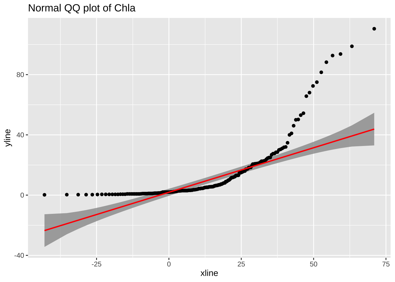
median(algae$Chla, na.rm = TRUE)[1] 5.475mean(algae$Chla, na.rm = TRUE)[1] 13.9712Obviously, the mean is not a representative value for Chla. For this we will use median to fill all missing values in this attribute, instead of doing it one value at a time:
algae <- algae |>
  mutate(Chla = if_else(is.na(Chla), median(Chla, na.rm = TRUE), Chla))
Filling unknowns using linear regression
This method is used when two variables are highly correlated. One value of variable A can be used to predict the value for variable B using the linear regression model.
First let’s see what variables in algae are highly correlated:
algae_numeric <- algae[, 4:18] %>%
  drop_na()  # Removes rows with NA values

cor_matrix <- algae_numeric |> correlate() |> plot()
cor_matrix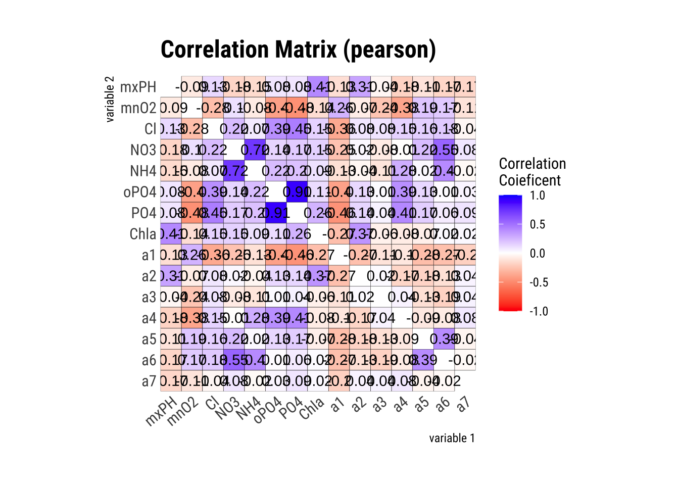
# study only the numerical variables (4-18) and use only the complete observations -- obs with NAs are not used. symnum() makes the correlation matrix more readableWe can see from the matrix, PO4 and oPO4 are correct with a confidence level of 90%.
Next, we find the linear model between PO4 and oPO4:
algae <- algae %>%
  filter(rowSums(is.na(.)) / ncol(.) < 0.2)#this is a method provided that selects the observations with 20% or move values as NAs.

m = lm(PO4 ~ oPO4, data = algae)
lm(formula = PO4 ~ oPO4, data = algae)
Call:
lm(formula = PO4 ~ oPO4, data = algae)

Coefficients:
(Intercept)         oPO4
     42.897        1.293
Check the model, is it good? See http://r-statistics.co/Linear-Regression.html
m |>
  summary()
Call:
lm(formula = PO4 ~ oPO4, data = algae)

Residuals:
    Min      1Q  Median      3Q     Max
-110.12  -36.34  -12.68   23.26  216.98

Coefficients:
            Estimate Std. Error t value Pr(>|t|)
(Intercept)   42.897      4.808   8.922 3.34e-16 ***
oPO4           1.293      0.041  31.535  < 2e-16 ***
---
Signif. codes:  0 '***' 0.001 '**' 0.01 '*' 0.05 '.' 0.1 ' ' 1

Residual standard error: 52.37 on 195 degrees of freedom
  (1 observation deleted due to missingness)
Multiple R-squared:  0.8361,    Adjusted R-squared:  0.8352
F-statistic: 994.5 on 1 and 195 DF,  p-value: < 2.2e-16
or…
m |>
  summary() |>
  tidy()
# A tibble: 2 × 5
term estimate std.error statistic p.value
<chr> <dbl> <dbl> <dbl> <dbl>
1 (Intercept) 42.9 4.81 8.92 3.34e-16
2 oPO4 1.29 0.0410 31.5 1.68e-78#tidy is from the tidymodels metapackage. This creates a more readable output for linear regressionsIf a good model, coefficients should all be significant (reject Ho coefficience is 0), Adjusted R-squared close to 1 (0.8 is very good).
F-statistics p-value should be less than the significant level (typically 0.05).
While R-squared provides an estimate of the strength of the relationship between your model and the response variable, it does not provide a formal hypothesis test for this relationship.
The F-test of overall significance determines whether this relationship is statistically significant.
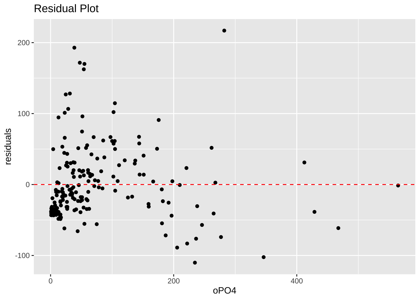
This model is good. We can also assess the fitness of the model with fitted line plot (should show the good fit), residual plot (should show residual being random).
This lm is PO4 = 1.293*oPO4 + 42.897
algae$PO4 [1] 170.000 558.750 187.057 138.700 97.580 56.667 111.750 77.434 71.000
[10] 46.600 20.750 19.000 17.000 15.000 61.600 98.250 50.000 57.833
[19] 61.500 771.600 586.000 18.000 40.000 27.500 11.500 44.136 13.600
[28] NA 45.000 19.000 142.000 304.000 130.750 47.000 23.000 84.460
[37] 3.000 3.000 253.250 255.280 296.000 175.046 344.600 326.857 40.667
[46] 43.500 39.000 6.000 121.000 20.812 49.333 22.900 11.800 11.818
[55] 6.500 1.000 4.000 6.000 11.000 6.000 14.000 6.667 6.750
[64] 7.200 6.000 10.750 2.500 351.600 313.600 279.066 152.333 58.623
[73] 249.250 233.500 215.500 102.333 105.727 111.375 108.000 56.667 60.000
[82] 104.000 69.930 214.000 254.600 169.001 607.167 624.733 303.333 391.750
[91] 265.250 232.833 244.000 218.000 138.500 239.000 235.667 205.875 211.667
[100] 186.500 154.125 183.667 292.625 285.714 201.778 275.143 124.200 141.833
[109] 132.546 17.333 26.000 16.662 102.571 86.997 10.111 18.293 13.200
[118] 432.909 320.400 287.000 262.727 222.286 122.000 127.222 89.625 284.000
[127] 277.333 177.625 72.900 82.444 66.750 173.750 317.000 84.000 213.000
[136] 88.500 115.000 98.143 143.750 197.143 35.200 23.485 200.231 147.833
[145] 276.000 123.333 75.207 116.200 188.667 72.696 116.200 34.000 76.333
[154] 58.374 361.000 236.000 125.800 54.916 75.333 186.000 252.500 269.667
[163] 46.438 85.000 171.272 232.900 146.452 246.667 219.909 272.222 388.167
[172] 167.900 137.778 194.100 221.278 21.300 11.000 14.354 7.000 6.200
[181] 7.654 16.000 56.091 52.875 228.364 85.400 87.125 101.455 127.000
[190] 81.558 50.455 120.889 91.111 61.444 79.750 75.904 140.220 140.517PO4 for observation 28 can then be filled with predicated value using the model
algae <- algae %>%
  mutate(PO4 = ifelse(row_number() == 28, 42.897 + 1.293 * oPO4, PO4))
res = resid(m)
oPO4_reduced <- algae %>%
filter(row_number() != 28) %>%
pull(oPO4)ggplot(data = data.frame(oPO4 = m$model$oPO4, res = res), aes(x = oPO4, y = res)) +
geom_point() +
geom_hline(yintercept = 0, linetype = "dashed", color = "red") +
labs(
x = "oPO4",
y = "residuals",
title = "Residual Plot"
)
If there are more PO4 cells to fill, we can use sapply() to apply this transformation to a set of values
Create a simple function fillPO4:
fillPO4 <- function(x) {
  if_else(is.na(x), 42.897 + 1.293 * x, x)
}
#if x is not NA, return 42.897+1.293*x algae[is.na(algae$PO4), "PO4"] <- sapply(algae[is.na(algae$PO4), "oPO4"], fillPO4)Apply calls fillPO4 function repeatedly, each time using one value in algae[is.na(algae$PO4), "oPO4"] as an argument.
You can perform a similar operation on subsets of observations. For example, if PO4 is missing for data collected in summer and season affects PO4 values, you may consider to use a linear model constructed with summer data only to obtain a more accurate prediction of PO4 from oPO4.
Filling unknowns by exploring similarities among cases
data(algae, package="DMwR2")
algae <- algae[-manyNAs(algae), ]
DM2R2 provides a method call knnImputation(). This method use the Euclidean distance to find the ten most similar cases of any water sample with some unknown value in a variable, and then use their values to fill in the unknown.
We can simply calculate the median of the values of the ten nearest neighbors to fill in the gaps. In case of unknown nominal variables (which do not occur in our algae data set), we would use the most frequent value (the mode) among the neighbors. The second method uses a weighted average of the values of the neighbors.
The weights decrease as the distance to the case of the neighbors increases.
algae <- knnImputation(algae, k = 10) #use the weighted average of k most similar samples


data(algae, package="DMwR2") #get data again so there are unknown values
algae <- algae[-manyNAs(algae), ]
algae <- knnImputation(algae, k = 10, meth="median") #use the median of k most similar samples
To see what is in knnImputation() (You are not required to read and understand the code):
getAnywhere(knnImputation())A single object matching 'knnImputation' was found
It was found in the following places
package:DMwR2
namespace:DMwR2
with value
function (data, k = 10, scale = TRUE, meth = "weighAvg", distData = NULL)
{
n <- nrow(data)
if (!is.null(distData)) {
distInit <- n + 1
data <- rbind(data, distData)
}
else distInit <- 1
N <- nrow(data)
ncol <- ncol(data)
contAttrs <- which(vapply(data, dplyr::type_sum, character(1)) %in%
c("dbl", "int"))
nomAttrs <- setdiff(seq.int(ncol), contAttrs)
hasNom <- length(nomAttrs)
dm <- data
if (scale)
dm[, contAttrs] <- scale(dm[, contAttrs])
if (hasNom)
for (i in nomAttrs) dm[[i]] <- as.integer(dm[[i]])
dm <- as.matrix(dm)
nas <- which(!complete.cases(dm))
if (!is.null(distData))
tgt.nas <- nas[nas <= n]
else tgt.nas <- nas
if (length(tgt.nas) == 0)
warning("No case has missing values. Stopping as there is nothing to do.")
xcomplete <- dm[setdiff(distInit:N, nas), ]
if (nrow(xcomplete) < k)
stop("Not sufficient complete cases for computing neighbors.")
for (i in tgt.nas) {
tgtAs <- which(is.na(dm[i, ]))
dist <- scale(xcomplete, dm[i, ], FALSE)
xnom <- setdiff(nomAttrs, tgtAs)
if (length(xnom))
dist[, xnom] <- ifelse(dist[, xnom] > 0, 1, dist[,
xnom])
dist <- dist[, -tgtAs]
dist <- sqrt(drop(dist^2 %*% rep(1, ncol(dist))))
ks <- order(dist)[seq(k)]
for (j in tgtAs) if (meth == "median")
data[i, j] <- centralValue(data[setdiff(distInit:N,
nas)[ks], j])
else data[i, j] <- centralValue(data[setdiff(distInit:N,
nas)[ks], j], exp(-dist[ks]))
}
data[1:n, ]
}
<bytecode: 0x13b5a13e8>
<environment: namespace:DMwR2>Scaling and normalization
Normalize value x: \(y = (x-mean)/standard_deviation(x)\) using scale()
Normalize values in penguins dataset:
library(dplyr)
library(palmerpenguins)
Attaching package: 'palmerpenguins'The following object is masked from 'package:modeldata':
penguinsdata(penguins)# select only numeric columns
penguins_numeric <- select(penguins, bill_length_mm, bill_depth_mm, flipper_length_mm, body_mass_g)
# normalize numeric columns
penguins_norm <- scale(penguins_numeric)
# convert back to data frame and add species column
peng.norm <- cbind(as.data.frame(penguins_norm), species = penguins$species)
# because scale() takes numeric matrix as input, we first remove Species column, then use cbind() to add the column back after normalization.summary(penguins) species island bill_length_mm bill_depth_mm
Adelie :152 Biscoe :168 Min. :32.10 Min. :13.10
Chinstrap: 68 Dream :124 1st Qu.:39.23 1st Qu.:15.60
Gentoo :124 Torgersen: 52 Median :44.45 Median :17.30
Mean :43.92 Mean :17.15
3rd Qu.:48.50 3rd Qu.:18.70
Max. :59.60 Max. :21.50
NA's :2 NA's :2
flipper_length_mm body_mass_g sex year
Min. :172.0 Min. :2700 female:165 Min. :2007
1st Qu.:190.0 1st Qu.:3550 male :168 1st Qu.:2007
Median :197.0 Median :4050 NA's : 11 Median :2008
Mean :200.9 Mean :4202 Mean :2008
3rd Qu.:213.0 3rd Qu.:4750 3rd Qu.:2009
Max. :231.0 Max. :6300 Max. :2009
NA's :2 NA's :2 summary(peng.norm) bill_length_mm bill_depth_mm flipper_length_mm body_mass_g
Min. :-2.16535 Min. :-2.05144 Min. :-2.0563 Min. :-1.8726
1st Qu.:-0.86031 1st Qu.:-0.78548 1st Qu.:-0.7762 1st Qu.:-0.8127
Median : 0.09672 Median : 0.07537 Median :-0.2784 Median :-0.1892
Mean : 0.00000 Mean : 0.00000 Mean : 0.0000 Mean : 0.0000
3rd Qu.: 0.83854 3rd Qu.: 0.78430 3rd Qu.: 0.8594 3rd Qu.: 0.6836
Max. : 2.87166 Max. : 2.20217 Max. : 2.1395 Max. : 2.6164
NA's :2 NA's :2 NA's :2 NA's :2
species
Adelie :152
Chinstrap: 68
Gentoo :124
scale() can also take an argument for center and an argument of scale to normalize data in some other ways, for example, \(y = (x-min)/(max-min)\)
max <- apply(select(penguins, -species), 2, max, na.rm=TRUE)
min <- apply(select(penguins, -species), 2, min, na.rm=TRUE)
max island bill_length_mm bill_depth_mm flipper_length_mm
"Torgersen" "59.6" "21.5" "231"
body_mass_g sex year
"6300" "male" "2009" min island bill_length_mm bill_depth_mm flipper_length_mm
"Biscoe" "32.1" "13.1" "172"
body_mass_g sex year
"2700" "female" "2007" # min-max normalization
penguin_scaled <- as.data.frame(lapply(penguins_numeric, function(x) (x - min(x, na.rm = TRUE)) / (max(x, na.rm = TRUE) - min(x, na.rm = TRUE))))
penguin_scaled <- cbind(penguins_norm, species = penguins$species)
summary(penguin_scaled) bill_length_mm bill_depth_mm flipper_length_mm body_mass_g
Min. :-2.16535 Min. :-2.05144 Min. :-2.0563 Min. :-1.8726
1st Qu.:-0.86031 1st Qu.:-0.78548 1st Qu.:-0.7762 1st Qu.:-0.8127
Median : 0.09672 Median : 0.07537 Median :-0.2784 Median :-0.1892
Mean : 0.00000 Mean : 0.00000 Mean : 0.0000 Mean : 0.0000
3rd Qu.: 0.83854 3rd Qu.: 0.78430 3rd Qu.: 0.8594 3rd Qu.: 0.6836
Max. : 2.87166 Max. : 2.20217 Max. : 2.1395 Max. : 2.6164
NA's :2 NA's :2 NA's :2 NA's :2
species
Min. :1.000
1st Qu.:1.000
Median :2.000
Mean :1.919
3rd Qu.:3.000
Max. :3.000
Discretizing variables (binning)
The process of transferring continuous functions, models, variables, and equations into discrete counterparts
Use dlookr’s binning(type = "equal") for equal-length cuts (bins)
Use Hmisc’s cut2() for equal-depth cuts
Boston Housing data as an example:
data(Boston, package="MASS")
summary(Boston$age)
Min. 1st Qu. Median Mean 3rd Qu. Max.
2.90 45.02 77.50 68.57 94.08 100.00 Boston$newAge <- dlookr::binning(Boston$age, 5, type = "equal") #create 5 bins and add new column newAge to Boston
summary(Boston$newAge) levels freq rate
1 [2.9,22.32] 45 0.08893281
2 (22.32,41.74] 71 0.14031621
3 (41.74,61.16] 70 0.13833992
4 (61.16,80.58] 81 0.16007905
5 (80.58,100] 239 0.47233202Boston$newAge <- dlookr::binning(Boston$age, nbins = 5, labels = c("very-young", "young", "mid", "older", "very-old"), type = "equal") #add labels
summary(Boston$newAge) levels freq rate
1 very-young 45 0.08893281
2 young 71 0.14031621
3 mid 70 0.13833992
4 older 81 0.16007905
5 very-old 239 0.47233202Equal-depth
install.packages("Hmisc")
library(Hmisc)
Boston$newAge <- cut2(Boston$age, g = 5) #create 5 equal-depth bins and add new column newAge to Boston

table(Boston$newAge)
Attaching package: 'Hmisc'The following object is masked from 'package:parsnip':
translateThe following objects are masked from 'package:dplyr':
src, summarizeThe following object is masked from 'package:dlookr':
describeThe following objects are masked from 'package:base':
format.pval, units
[ 2.9, 38.1) [38.1, 66.1) [66.1, 86.1) [86.1, 95.7) [95.7,100.0]
         102          101          101          101          101
Assign labels
Boston$newAge <- factor(cut2(Boston$age, g = 5), labels = c("very-young", "young", "mid", "older", "very-old"))

table(Boston$newAge)
very-young      young        mid      older   very-old
       102        101        101        101        101
Plot an equal-width histogram of width 10:
hist(Boston$age, breaks = seq(0, 101,by = 10)) #seq() gives the function for breaks. The age ranges from 0 – 101.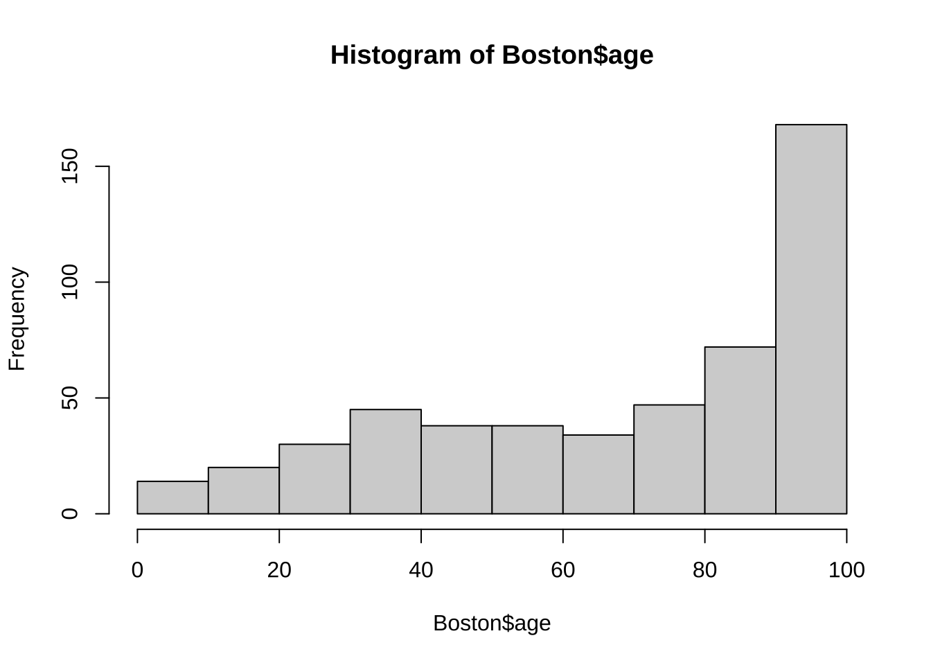
or, use ggplot2!
library(ggplot2)

Boston |>
  ggplot(aes(x = age)) +
  geom_histogram(binwidth = 10)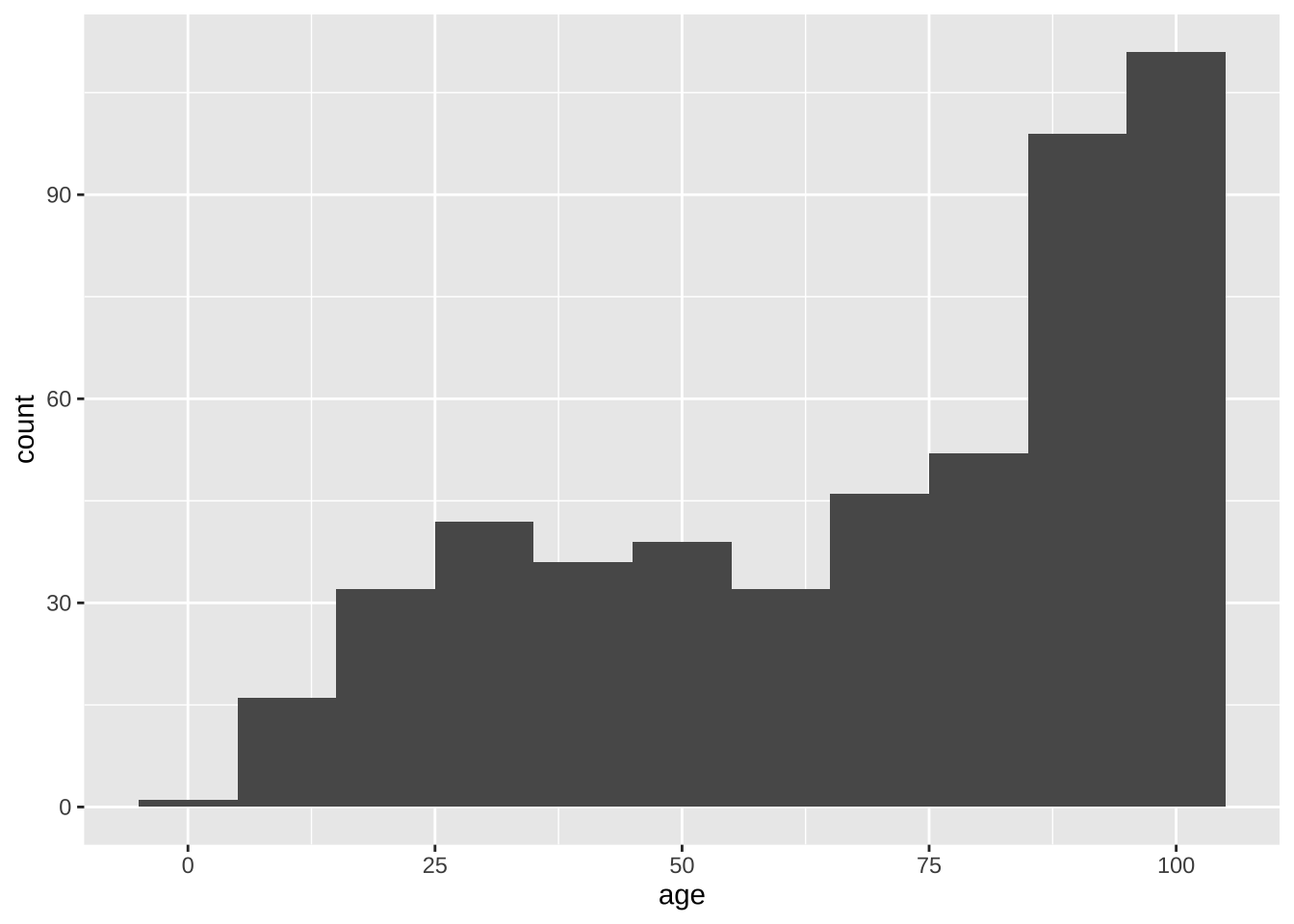
dlookr also has great binning functions you can try!
https://choonghyunryu.github.io/dlookr/reference/binning.html
Decimal scaling
data <- c(10, 20, 30, 50, 100)(nDigits = nchar(max(abs(data)))) #nchar counts the number of characters[1] 3(decimalScale = data / (10^nDigits))[1] 0.01 0.02 0.03 0.05 0.10Smoothing by bin mean
age = c(13, 15, 16, 16, 19, 20, 20, 21, 22, 22, 25, 25, 25, 25, 30)

# Separate data into bins of depth 3
(bins = matrix(age, nrow = length(age) / 5, byrow = TRUE))
[,1] [,2] [,3] [,4] [,5]
[1,] 13 15 16 16 19
[2,] 20 20 21 22 22
[3,] 25 25 25 25 30Find the average of each bin:
(bin_means = apply(bins, 1, FUN = mean))[1] 15.8 21.0 26.0Replace values with their bin mean:
for (i in 1:nrow(bins)) {
   bins[i,] = bin_means[i]
 }
bins
[,1] [,2] [,3] [,4] [,5]
[1,] 15.8 15.8 15.8 15.8 15.8
[2,] 21.0 21.0 21.0 21.0 21.0
[3,] 26.0 26.0 26.0 26.0 26.0(age_bin_mean_smoothed = round(as.vector(t(bins)), 2)) [1] 15.8 15.8 15.8 15.8 15.8 21.0 21.0 21.0 21.0 21.0 26.0 26.0 26.0 26.0 26.0Variable correlations and dimensionality reduction
Chi-squared test
H0: (Prisoner’s race)(Victim’s race) are independent.
data (contingency table):
racetable = rbind(c(151,9), c(63,103))
test1 = chisq.test(racetable, correct=F)
test1
    Pearson's Chi-squared test

data:  racetable
X-squared = 115.01, df = 1, p-value < 2.2e-16
p-value is less than 0.05: chance to get X-squared value of 115.01 assuming H0 is true is very slim (close to 0), so reject H0.
Loglinear model
Extending chi-squared to more than 2 categorical variables.
Loglinear models model cell counts in contingency tables.
Adapted from https://data.library.virginia.edu/an-introduction-to-loglinear-models/:
Data from Agresti (1996, Table 6.3) modified. It summarizes responses from a survey that asked high school seniors in a particular city whether they had ever used alcohol, cigarettes, or marijuana. A categorical variable age is added.
We’re interested in how the cell counts in the contingency table depend on the levels of the categorical variables.
Get the data in. We will be analyzing cells in contingency tables, so use a multi-dimensional array to hold the data.
seniors <- array(data = c(911, 44, 538, 456, 3, 2, 43, 279, 911, 44, 538, 456, 3, 2, 43, 279),
                  dim = c(2, 2, 2, 2),
                  dimnames = list("cigarette" = c("yes", "no"),
                                  "marijuana" = c("yes", "no"),
                                  "alcohol" = c("yes", "no"),
                                  "age" =c("younger", "older")))
Observe how data is saved in the 2x2x2x2 array:
seniors, , alcohol = yes, age = younger
marijuana
cigarette yes no
yes 911 538
no 44 456
, , alcohol = no, age = younger
marijuana
cigarette yes no
yes 3 43
no 2 279
, , alcohol = yes, age = older
marijuana
cigarette yes no
yes 911 538
no 44 456
, , alcohol = no, age = older
marijuana
cigarette yes no
yes 3 43
no 2 279Next, do loglinear modeling using the glm function (generalized linear models).
We need to convert the array to a table then to a data frame.
Calling as.data.frame on a table object in R returns a data frame with a column for cell frequencies where each row represents a unique combination of variables.
seniors.tb <- as.table(seniors)
seniors.tb
, , alcohol = yes, age = younger
marijuana
cigarette yes no
yes 911 538
no 44 456
, , alcohol = no, age = younger
marijuana
cigarette yes no
yes 3 43
no 2 279
, , alcohol = yes, age = older
marijuana
cigarette yes no
yes 911 538
no 44 456
, , alcohol = no, age = older
marijuana
cigarette yes no
yes 3 43
no 2 279seniors.df <- as.data.frame(seniors.tb)
seniors.df cigarette marijuana alcohol age Freq
1 yes yes yes younger 911
2 no yes yes younger 44
3 yes no yes younger 538
4 no no yes younger 456
5 yes yes no younger 3
6 no yes no younger 2
7 yes no no younger 43
8 no no no younger 279
9 yes yes yes older 911
10 no yes yes older 44
11 yes no yes older 538
12 no no yes older 456
13 yes yes no older 3
14 no yes no older 2
15 yes no no older 43
16 no no no older 279Next, we model Freq (this is the count in the contingency table) as a function of the three variables using the glm function. Set family = poisson because we are assuming independent counts.
Poisson distribution: discrete probability distribution that expresses the probability of a given number of events occurring in a fixed interval of time or space if these events occur with a known constant rate and independently of the time since the last event.
Our H0 is the four variables are independent of one another.
We will test the saturated model first (including all variables and all two-way and three-way interactions), because it will show the significance for all variables and their interactions
Use * to connect all variables to get a saturated model, which will fit the data perfectly. Then we will remove effects that are not significant.
mod.S4 <- glm(Freq ~ (cigarette * marijuana * alcohol * age), data = seniors.df, family=poisson)
summary(mod.S4)
Call:
glm(formula = Freq ~ (cigarette * marijuana * alcohol * age),
    family = poisson, data = seniors.df)

Coefficients:
                                             Estimate Std. Error z value
(Intercept)                                 6.815e+00  3.313e-02 205.682
cigaretteno                                -3.030e+00  1.544e-01 -19.633
marijuanano                                -5.267e-01  5.437e-02  -9.686
alcoholno                                  -5.716e+00  5.783e-01  -9.884
ageolder                                   -1.946e-15  4.685e-02   0.000
cigaretteno:marijuanano                     2.865e+00  1.670e-01  17.159
cigaretteno:alcoholno                       2.625e+00  9.258e-01   2.835
marijuanano:alcoholno                       3.189e+00  5.996e-01   5.319
cigaretteno:ageolder                        7.281e-15  2.183e-01   0.000
marijuanano:ageolder                        1.351e-15  7.690e-02   0.000
alcoholno:ageolder                          2.098e-15  8.178e-01   0.000
cigaretteno:marijuanano:alcoholno          -5.895e-01  9.424e-01  -0.626
cigaretteno:marijuanano:ageolder           -6.706e-15  2.361e-01   0.000
cigaretteno:alcoholno:ageolder             -3.770e-15  1.309e+00   0.000
marijuanano:alcoholno:ageolder             -1.143e-15  8.480e-01   0.000
cigaretteno:marijuanano:alcoholno:ageolder  3.239e-15  1.333e+00   0.000
                                           Pr(>|z|)
(Intercept)                                 < 2e-16 ***
cigaretteno                                 < 2e-16 ***
marijuanano                                 < 2e-16 ***
alcoholno                                   < 2e-16 ***
ageolder                                    1.00000
cigaretteno:marijuanano                     < 2e-16 ***
cigaretteno:alcoholno                       0.00458 **
marijuanano:alcoholno                      1.04e-07 ***
cigaretteno:ageolder                        1.00000
marijuanano:ageolder                        1.00000
alcoholno:ageolder                          1.00000
cigaretteno:marijuanano:alcoholno           0.53160
cigaretteno:marijuanano:ageolder            1.00000
cigaretteno:alcoholno:ageolder              1.00000
marijuanano:alcoholno:ageolder              1.00000
cigaretteno:marijuanano:alcoholno:ageolder  1.00000
---
Signif. codes:  0 '***' 0.001 '**' 0.01 '*' 0.05 '.' 0.1 ' ' 1

(Dispersion parameter for poisson family taken to be 1)

    Null deviance: 5.7029e+03  on 15  degrees of freedom
Residual deviance: 8.7041e-14  on  0  degrees of freedom
AIC: 130.09

Number of Fisher Scoring iterations: 3Note: “Residual deviance” indicates the fitness of the model to the data. A good fit would have residual deviance less than or close to its degree of freedom. That is the case for the saturated model, which is expected.
Then look at “Coefficients” (these are the lamdas). Many of them are not significant (*, **, *** indicates significant lamdas)
By examining those insignificant effects, we see they all involve age.
Now lets’ remove age and re-generate a model with the remaining three variables.
mod.S3 <- glm(Freq ~ (cigarette * marijuana * alcohol), data = seniors.df, family = poisson)
summary(mod.S3)
Call:
glm(formula = Freq ~ (cigarette * marijuana * alcohol), family = poisson,
    data = seniors.df)

Coefficients:
                                  Estimate Std. Error z value Pr(>|z|)
(Intercept)                        6.81454    0.02343 290.878  < 2e-16 ***
cigaretteno                       -3.03035    0.10914 -27.765  < 2e-16 ***
marijuanano                       -0.52668    0.03845 -13.699  < 2e-16 ***
alcoholno                         -5.71593    0.40892 -13.978  < 2e-16 ***
cigaretteno:marijuanano            2.86499    0.11806  24.267  < 2e-16 ***
cigaretteno:alcoholno              2.62489    0.65466   4.010 6.08e-05 ***
marijuanano:alcoholno              3.18927    0.42400   7.522 5.40e-14 ***
cigaretteno:marijuanano:alcoholno -0.58951    0.66635  -0.885    0.376
---
Signif. codes:  0 '***' 0.001 '**' 0.01 '*' 0.05 '.' 0.1 ' ' 1

(Dispersion parameter for poisson family taken to be 1)

    Null deviance:  5.7029e+03  on 15  degrees of freedom
Residual deviance: -1.7897e-13  on  8  degrees of freedom
AIC: 114.09

Number of Fisher Scoring iterations: 3
We see the model fits well, and most effects are significant now.
The insignificant one is the 3-way interaction among the three factors
For data reduction, we are done – we removed age variable. Because all cigarette, marijuana, and alcohol effects are significant, we can’t remove any of these from the data set, even though the 3-way interaction is not significant.
For data modeling, we can remove the 3-way interaction by testing “Freq ~ (cigarette + marijuana + alcohol)^2” (^2 tells glm to check only two way interactions).
mod.3 <- glm(Freq ~ (cigarette + marijuana + alcohol)^2, data = seniors.df, family = poisson)
summary(mod.3)
Call:
glm(formula = Freq ~ (cigarette + marijuana + alcohol)^2, family = poisson,
    data = seniors.df)

Coefficients:
                        Estimate Std. Error z value Pr(>|z|)
(Intercept)              6.81387    0.02342 290.902   <2e-16 ***
cigaretteno             -3.01575    0.10721 -28.130   <2e-16 ***
marijuanano             -0.52486    0.03838 -13.674   <2e-16 ***
alcoholno               -5.52827    0.31976 -17.289   <2e-16 ***
cigaretteno:marijuanano  2.84789    0.11585  24.582   <2e-16 ***
cigaretteno:alcoholno    2.05453    0.12308  16.692   <2e-16 ***
marijuanano:alcoholno    2.98601    0.32858   9.088   <2e-16 ***
---
Signif. codes:  0 '***' 0.001 '**' 0.01 '*' 0.05 '.' 0.1 ' ' 1

(Dispersion parameter for poisson family taken to be 1)

    Null deviance: 5702.92195  on 15  degrees of freedom
Residual deviance:    0.74797  on  9  degrees of freedom
AIC: 112.83

Number of Fisher Scoring iterations: 4
Now compare the fitted and observed values and see how well they match up:
cbind(mod.3$data, fitted(mod.3)) cigarette marijuana alcohol age Freq fitted(mod.3)
1 yes yes yes younger 911 910.38317
2 no yes yes younger 44 44.61683
3 yes no yes younger 538 538.61683
4 no no yes younger 456 455.38317
5 yes yes no younger 3 3.61683
6 no yes no younger 2 1.38317
7 yes no no younger 43 42.38317
8 no no no younger 279 279.61683
9 yes yes yes older 911 910.38317
10 no yes yes older 44 44.61683
11 yes no yes older 538 538.61683
12 no no yes older 456 455.38317
13 yes yes no older 3 3.61683
14 no yes no older 2 1.38317
15 yes no no older 43 42.38317
16 no no no older 279 279.61683They fit well!
Correlations
library(tidyr) # data manipulation
penguins_numeric |>
  drop_na() |>
  correlate()
# A tibble: 12 × 3
var1 var2 coef_corr
<fct> <fct> <dbl>
1 bill_depth_mm bill_length_mm -0.235
2 flipper_length_mm bill_length_mm 0.656
3 body_mass_g bill_length_mm 0.595
4 bill_length_mm bill_depth_mm -0.235
5 flipper_length_mm bill_depth_mm -0.584
6 body_mass_g bill_depth_mm -0.472
7 bill_length_mm flipper_length_mm 0.656
8 bill_depth_mm flipper_length_mm -0.584
9 body_mass_g flipper_length_mm 0.871
10 bill_length_mm body_mass_g 0.595
11 bill_depth_mm body_mass_g -0.472
12 flipper_length_mm body_mass_g 0.871bill_length_mm and flipper_length_mm are highly negatively correlated, body_mass_g and flipper_length_mm are strongly positively correlated as well.
Principal components analysis (PCA)
pca.data <- penguins |>
  drop_na() |>
  select(-species, -island, -sex)

pca <- princomp(pca.data)
loadings(pca)
Loadings:
                  Comp.1 Comp.2 Comp.3 Comp.4 Comp.5
bill_length_mm            0.319  0.941  0.108
bill_depth_mm                    0.144 -0.984
flipper_length_mm         0.943 -0.304 -0.125
body_mass_g        1.000
year                                           0.997

               Comp.1 Comp.2 Comp.3 Comp.4 Comp.5
SS loadings       1.0    1.0    1.0    1.0    1.0
Proportion Var    0.2    0.2    0.2    0.2    0.2
Cumulative Var 0.2 0.4 0.6 0.8 1.0head(pca$scores) # pca result is a list, and the component scores are elements in the list Comp.1 Comp.2 Comp.3 Comp.4 Comp.5
[1,] -457.3251 -13.376298 1.24790414 0.3764738 -0.5892777
[2,] -407.2522 -9.205245 -0.03266674 1.0902167 -0.6935631
[3,] -957.0447 8.128321 -2.49146655 -0.7208225 -1.3723988
[4,] -757.1158 1.838910 -4.88056871 -2.0736684 -1.3477178
[5,] -557.1773 -3.416994 -1.12926657 -2.6292970 -1.1451328
[6,] -582.3093 -11.398030 0.80239704 1.1987261 -0.5976776If we are happy with capturing 75% of the original variance of the cases, we can reduce the original data to the first three components.
Component scores are computed based on the loading, for example:
comp3 = 0.941*bill_length_mm + 0.144*``bill_depth_mm``- 0.309*flipper_length_mm
penguins_na <- penguins |>
  drop_na()

peng.reduced <- data.frame(pca$scores[,1:3], Species = penguins_na$species)

head(peng.reduced)
Comp.1 Comp.2 Comp.3 Species
1 -457.3251 -13.376298 1.24790414 Adelie
2 -407.2522 -9.205245 -0.03266674 Adelie
3 -957.0447 8.128321 -2.49146655 Adelie
4 -757.1158 1.838910 -4.88056871 Adelie
5 -557.1773 -3.416994 -1.12926657 Adelie
6 -582.3093 -11.398030 0.80239704 AdelieNow we can use peng.reduced data frame for subsequent analyses:
Haar Discrete Wavelet Transform, using the example shown in class
Output:
| W: | A list with element i comprised of a matrix containing the ith level wavelet coefficients (differences) |
| V: | A list with element i comprised of a matrix containing the ith level scaling coefficients (averages). |
install.packages("wavelets")
library(wavelets)
Attaching package: 'wavelets'The following object is masked from 'package:car':
dwtx <- c(2, 2, 0, 2, 3, 5, 4, 4)
wt <- dwt(x,filter="haar", n.levels = 3) #with 8-element vector, 3 level is the max.
wtAn object of class "dwt"
Slot "W":
$W1
[,1]
[1,] 0.000000
[2,] 1.414214
[3,] 1.414214
[4,] 0.000000
$W2
[,1]
[1,] -1
[2,] 0
$W3
[,1]
[1,] 3.535534
Slot "V":
$V1
[,1]
[1,] 2.828427
[2,] 1.414214
[3,] 5.656854
[4,] 5.656854
$V2
[,1]
[1,] 3
[2,] 8
$V3
[,1]
[1,] 7.778175
Slot "filter":
Filter Class: Daubechies
Name: HAAR
Length: 2
Level: 1
Wavelet Coefficients: 7.0711e-01 -7.0711e-01
Scaling Coefficients: 7.0711e-01 7.0711e-01
Slot "level":
[1] 3
Slot "n.boundary":
[1] 0 0 0
Slot "boundary":
[1] "periodic"
Slot "series":
[,1]
[1,] 2
[2,] 2
[3,] 0
[4,] 2
[5,] 3
[6,] 5
[7,] 4
[8,] 4
Slot "class.X":
[1] "numeric"
Slot "attr.X":
list()
Slot "aligned":
[1] FALSE
Slot "coe":
[1] FALSEWhy aren’t the W and V vectors having the same values as shown in class?
Because in class, use simply taking the average and differences/2, in the default Haar, the default coefficients are sqrt(2)/2, see the section in bold above.
Reconstruct the original:
idwt(wt)[1] 2 2 0 2 3 5 4 4Obtain transform results as shown in class, use a different filter:
xt = dwt(x, filter = wt.filter(c(0.5, -0.5)), n.levels = 3)
xt
An object of class "dwt"
Slot "W":
$W1
[,1]
[1,] 0
[2,] 1
[3,] 1
[4,] 0
$W2
[,1]
[1,] -0.5
[2,] 0.0
$W3
[,1]
[1,] 1.25
Slot "V":
$V1
[,1]
[1,] 2
[2,] 1
[3,] 4
[4,] 4
$V2
[,1]
[1,] 1.5
[2,] 4.0
$V3
[,1]
[1,] 2.75
Slot "filter":
Filter Class: none
Name: NONE
Length: 2
Level: 1
Wavelet Coefficients: 5.0000e-01 -5.0000e-01
Scaling Coefficients: 5.0000e-01 5.0000e-01
Slot "level":
[1] 3
Slot "n.boundary":
[1] 0 0 0
Slot "boundary":
[1] "periodic"
Slot "series":
[,1]
[1,] 2
[2,] 2
[3,] 0
[4,] 2
[5,] 3
[6,] 5
[7,] 4
[8,] 4
Slot "class.X":
[1] "numeric"
Slot "attr.X":
list()
Slot "aligned":
[1] FALSE
Slot "coe":
[1] FALSEReconstruct the original:
idwt(xt)[1] 0.3125 0.3125 -0.4375 0.5625 0.0000 1.0000 0.5000 0.5000Sampling
set.seed(1)
age <- c(25, 25, 25, 30, 33, 33, 35, 40, 45, 46, 52, 70)
Simple random sampling, without replacement:
sample(age, 5)[1] 45 30 35 25 25Simple random sampling, with replacement:
sample(age, 5, replace = TRUE)[1] 35 52 25 52 25Stratified sampling
library(dplyr)
set.seed(1) #make results the same each run
summary(algae)
season size speed mxPH mnO2
autumn:40 large :44 high :84 Min. :5.600 Min. : 1.500
spring:53 medium:84 low :33 1st Qu.:7.705 1st Qu.: 7.825
summer:44 small :70 medium:81 Median :8.060 Median : 9.800
winter:61 Mean :8.019 Mean : 9.135
3rd Qu.:8.400 3rd Qu.:10.800
Max. :9.700 Max. :13.400
Cl NO3 NH4 oPO4
Min. : 0.222 Min. : 0.050 Min. : 5.00 Min. : 1.00
1st Qu.: 10.425 1st Qu.: 1.296 1st Qu.: 38.33 1st Qu.: 15.70
Median : 32.178 Median : 2.675 Median : 103.17 Median : 40.15
Mean : 42.434 Mean : 3.282 Mean : 501.30 Mean : 73.59
3rd Qu.: 57.492 3rd Qu.: 4.446 3rd Qu.: 226.95 3rd Qu.: 99.33
Max. :391.500 Max. :45.650 Max. :24064.00 Max. :564.60
PO4 Chla a1 a2
Min. : 1.00 Min. : 0.200 Min. : 0.000 Min. : 0.000
1st Qu.: 41.38 1st Qu.: 2.000 1st Qu.: 1.525 1st Qu.: 0.000
Median :103.29 Median : 5.155 Median : 6.950 Median : 3.000
Mean :137.88 Mean : 13.355 Mean :16.996 Mean : 7.471
3rd Qu.:213.75 3rd Qu.: 17.200 3rd Qu.:24.800 3rd Qu.:11.275
Max. :771.60 Max. :110.456 Max. :89.800 Max. :72.600
a3 a4 a5 a6
Min. : 0.000 Min. : 0.000 Min. : 0.000 Min. : 0.000
1st Qu.: 0.000 1st Qu.: 0.000 1st Qu.: 0.000 1st Qu.: 0.000
Median : 1.550 Median : 0.000 Median : 2.000 Median : 0.000
Mean : 4.334 Mean : 1.997 Mean : 5.116 Mean : 6.005
3rd Qu.: 4.975 3rd Qu.: 2.400 3rd Qu.: 7.500 3rd Qu.: 6.975
Max. :42.800 Max. :44.600 Max. :44.400 Max. :77.600
a7
Min. : 0.000
1st Qu.: 0.000
Median : 1.000
Mean : 2.487
3rd Qu.: 2.400
Max. :31.600 sample <-algae |> group_by(season) |> sample_frac(0.25)
summary(sample) season size speed mxPH mnO2
autumn:10 large :18 high :16 Min. :5.600 Min. : 1.500
spring:13 medium:20 low :13 1st Qu.:7.840 1st Qu.: 8.200
summer:11 small :11 medium:20 Median :8.100 Median : 9.700
winter:15 Mean :8.126 Mean : 9.084
3rd Qu.:8.500 3rd Qu.:10.800
Max. :9.700 Max. :11.800
Cl NO3 NH4 oPO4
Min. : 0.222 Min. :0.130 Min. : 5.00 Min. : 1.00
1st Qu.: 9.055 1st Qu.:0.921 1st Qu.: 43.75 1st Qu.: 21.08
Median : 28.333 Median :2.680 Median : 103.33 Median : 49.00
Mean : 39.175 Mean :2.794 Mean : 213.60 Mean : 78.49
3rd Qu.: 51.113 3rd Qu.:4.053 3rd Qu.: 225.00 3rd Qu.:125.67
Max. :173.750 Max. :6.640 Max. :1495.00 Max. :267.75
PO4 Chla a1 a2
Min. : 1.00 Min. : 0.300 Min. : 0.00 Min. : 0.00
1st Qu.: 69.93 1st Qu.: 2.500 1st Qu.: 1.20 1st Qu.: 1.50
Median :125.80 Median : 6.209 Median : 5.70 Median : 5.60
Mean :142.05 Mean : 14.848 Mean :17.94 Mean :10.24
3rd Qu.:228.36 3rd Qu.: 20.829 3rd Qu.:18.10 3rd Qu.:14.50
Max. :391.75 Max. :110.456 Max. :86.60 Max. :72.60
a3 a4 a5 a6
Min. : 0.000 Min. : 0.000 Min. : 0.000 Min. : 0.00
1st Qu.: 0.000 1st Qu.: 0.000 1st Qu.: 0.000 1st Qu.: 0.00
Median : 1.400 Median : 0.000 Median : 1.200 Median : 0.00
Mean : 3.498 Mean : 1.349 Mean : 4.678 Mean : 6.12
3rd Qu.: 4.000 3rd Qu.: 1.800 3rd Qu.: 7.700 3rd Qu.: 5.10
Max. :24.800 Max. :13.400 Max. :22.100 Max. :52.50
a7
Min. : 0.000
1st Qu.: 0.000
Median : 1.000
Mean : 2.367
3rd Qu.: 2.200
Max. :31.200 Cluster sampling
library(sampling)
age <- c(13, 15, 16, 16, 19, 20, 20, 21, 22, 22, 25, 25, 25, 25, 30, 33, 33, 35, 35, 35, 35, 36, 40, 45, 46, 52, 70)
s <- kmeans(age, 3) #cluster on age to form 3 clusters
s$cluster
[1] 3 3 3 3 3 2 2 2 2 2 2 2 2 2 2 1 1 1 1 1 1 1 1 1 1 1 1ageframe <- data.frame(age)
ageframe$condition <- s$cluster # add cluster label as condition
cluster(ageframe, clustername = "condition", size = 2) # select 2 clusters out of the threeWarning in cluster(ageframe, clustername = "condition", size = 2): the method
is not specified; by default, the method is srswor condition ID_unit Prob
1 1 16 0.6666667
2 1 17 0.6666667
3 1 18 0.6666667
4 1 19 0.6666667
5 1 20 0.6666667
6 1 21 0.6666667
7 1 22 0.6666667
8 1 23 0.6666667
9 1 24 0.6666667
10 1 25 0.6666667
11 1 26 0.6666667
12 1 27 0.6666667
13 3 1 0.6666667
14 3 4 0.6666667
15 3 5 0.6666667
16 3 2 0.6666667
17 3 3 0.6666667Handling Text Datasets
pacman::p_load(tm,
               SnowballC)#tm uses SnowballC for stemming
# read corpus
# Emails.csv,  holding some of Hillary's emails
data <- read.csv(here::here("data", "Emails.csv"), stringsAsFactors = FALSE)

docs <- Corpus(VectorSource(data$RawText))
mode(docs)
[1] "list"Inspect a document
docs[[20]]<<PlainTextDocument>>
Metadata: 7
Content: chars: 1150Preprocessing text
docs <- docs |>
         tm_map(removePunctuation) |>
         tm_map(content_transformer(tolower)) |> #to lower case
         tm_map(removeNumbers) |>
         tm_map(removeWords, stopwords("en")) |> #stopwords, such as a, an.
         tm_map(stripWhitespace) |>
         tm_map(stemDocument) #e.g. computer -> comput
Warning in tm_map.SimpleCorpus(docs, removePunctuation): transformation drops
documentsWarning in tm_map.SimpleCorpus(tm_map(docs, removePunctuation),
content_transformer(tolower)): transformation drops documentsWarning in tm_map.SimpleCorpus(tm_map(tm_map(docs, removePunctuation),
content_transformer(tolower)), : transformation drops documentsWarning in tm_map.SimpleCorpus(tm_map(tm_map(tm_map(docs, removePunctuation), :
transformation drops documentsWarning in tm_map.SimpleCorpus(tm_map(tm_map(tm_map(tm_map(docs,
removePunctuation), : transformation drops documentsWarning in tm_map.SimpleCorpus(tm_map(tm_map(tm_map(tm_map(tm_map(docs, :
transformation drops documentscontent(docs[[20]]) #note: stemming reduces a word to its ‘root’ with the aassumption that the ‘root’ represents the semantics of a word, e.g. computer, computing, computation, computers are about the concept of compute, which may be represented by ‘comput’. but stemming is never perfect.[1] "unclassifi us depart state case f doc c date state dept produc hous select benghazi comm subject agreement sensit inform redact foia waiver releas full sent subject amaz sullivan jacob j sullivaniistategov wednesday septemb pm sherman wendi r h mill cheryl d nuland victoria j rein philipp re youth libya sherman wendi r sent wednesday septemb pm idrdintonemailcom hdrgclintonemailcom mill cheryl d sullivan jacob nuland victoria rein philipp subject fw youth libya hope see pictur kamala sent lakhdhir kamala sent wednesday septemb pm sherman wendi r cc escrogima ana grantham chris w subject youth libya libya hurra tv via facebook unclassifi us depart state case f doc c date state dept produc hous select benghazi comm subject agreement sensit inform redact foia waiver statescb"Convert text to a matrix using TF*IDF scores (see TF*IDF scores in Han’s text):
DTData <- DocumentTermMatrix(docs, control = list(weighting = weightTfIdf))Warning in TermDocumentMatrix.SimpleCorpus(x, control): custom functions are
ignoredWarning in weighting(x): empty document(s): 1931DTData<<DocumentTermMatrix (documents: 7945, terms: 42473)>>
Non-/sparse entries: 885247/336562738
Sparsity : 100%
Maximal term length: 127
Weighting : term frequency - inverse document frequency (normalized) (tf-idf)inspect(DTData[1:2, 1:5])<<DocumentTermMatrix (documents: 2, terms: 5)>>
Non-/sparse entries: 7/3
Sparsity : 30%
Maximal term length: 9
Weighting : term frequency - inverse document frequency (normalized) (tf-idf)
Sample :
Terms
Docs agreement appreci arm benghazi boss
1 0.09372950 0.06292734 0.06305152 0.12828049 0.09281579
2 0.03236792 0.00000000 0.00000000 0.05062803 0.00000000Create term-document matrix (also called inverted index, see Han’s text in a later chapter):
TDData <- TermDocumentMatrix(docs, control = list(weighting = weightTfIdf))Warning in TermDocumentMatrix.SimpleCorpus(docs, control = list(weighting =
weightTfIdf)): custom functions are ignoredWarning in weighting(x): empty document(s): 1931inspect(TDData[1:2, 1:5])<<TermDocumentMatrix (terms: 2, documents: 5)>>
Non-/sparse entries: 6/4
Sparsity : 40%
Maximal term length: 9
Weighting : term frequency - inverse document frequency (normalized) (tf-idf)
Sample :
Docs
Terms 1 2 3 4 5
agreement 0.09372950 0.03236792 0.07881799 0.07580309 0.03906373
appreci 0.06292734 0.00000000 0.00000000 0.00000000 0.00000000Explore the dataset
findFreqTerms(TDData, lowfreq = 75, highfreq = 1000)[1] "abedin" "cheryl" "huma" "call"
[5] "abedinhstategov"Find correlations among terms:
findAssocs(TDData, terms = "bill", corlimit = 0.25)$bill
burn
0.26 findAssocs(DTData, terms=c("bill"), corlimit = 0.25)$bill
burn
0.26 findAssocs(DTData, terms=c("schedul"), corlimit = 0.3)$schedul
lona valmoro valmoroustategov
0.39 0.38 0.38 Create a word cloud
install.packages("wordcloud")
install.packages("RColorBrewer")
library(wordcloud)
Loading required package: RColorBrewerdata <- as.matrix(TDData)
freq <- sort(rowSums(data), decreasing = TRUE)
base <-data.frame(word = names(freq), freq = freq)png() opens a new device ‘png’ to output the graph to a local file:
png(file = "wordCloud.png", width = 1000, height = 700, bg= "grey30")

wordcloud(base$word, base$freq, col = terrain.colors(length(base$word), alpha = 0.9),
random.order = FALSE, rot.per = 0.3, scale = c(1, .1))
dev.off() closed the .png file, now the current display is the default display in RStudio. Use dev.list() to find the graphics devices that are active, repeatedly use dev.off() to close devices that not needed. R Studio is the default display. When all other devices are closed, the default display is used.
Output the graph to the default display in RStudio
wordcloud(base$word, base$freq, col = terrain.colors(length(base$word), alpha = 0.9),
random.order = FALSE, rot.per = 0.3, scale = c(1, .1))
Can you remove hrodclintonemailcom and redo the word cloud?
Sometimes you need to one-hot encoding a section of a dataframe. You can do it by using onehot package.
install.packages("onehot")
library(onehot)
d <- data.frame(language=c("javascript", "python", "java"), hours=c(10, 3, 5) )
d$language <- as.factor(d$language) #convert the column to be encoded to Factor
encoded <- onehot(d)
new_d <- predict(encoded, d)
new_d
language=java language=javascript language=python hours
[1,] 0 1 0 10
[2,] 0 0 1 3
[3,] 1 0 0 5One hot encoding for data frame with multi-value cells (language = "javascript, python")
install.packages("qdapTools")
library(qdapTools)
d <- data.frame(language=c("javascript, python", "java"), hours = c(3, 5) )
d
Attaching package: 'qdapTools'The following object is masked from 'package:dplyr':
id language hours
1 javascript, python 3
2 java 5dlist <- as.list(d)
new_d <- data.frame(cbind(dlist, mtabulate(strsplit(as.character(dlist$language), ", "))))
new_d language hours java javascript python
1 javascript, python 3 0 1 1
2 java 5 1 0 0[ADVANCED]
Exercises on your data set:
What attributes are there in your data set?
Do you have highly correlated attributes? How did you find out about the correlations or lack of correlations?
Do you have numerical attributes that you might want to bin? Try at least two methods and compare the differences.
If you have categorical attributes, use the concept hierarchy generation heuristics (based on attribute value counts) suggested in the textbook to produce some concept hierarchies. How well does this approach work for your attributes?