Classification: Alternative Techniques

Install packages

Install the packages used in this chapter:

if(!require(pacman))
  install.packages("pacman")

pacman::p_load(
  C50,                # C5.0 Decision Trees and Rule-Based Models
  caret,              # Classification and Regression Training
  e1071,              # Misc Functions of the Department of Statistics (e1071), TU Wien
  keras,              # R Interface to 'Keras'
  kernlab,            # Kernel-Based Machine Learning Lab
  lattice,            # Trellis Graphics for R
  MASS,               # Support Functions and Datasets for Venables and Ripley's MASS
  mlbench,            # Machine Learning Benchmark Problems
  nnet,               # Feedforward Neural Networks and Multinomial Log-Linear Models
  palmerpenguins,     # Palmer Archipelago (Antarctica) Penguin Data
  party,              # A Laboratory for Recursive Partytioning
  partykit,           # A Toolkit for Recursive Partytioning
  randomForest,       # Breiman and Cutler's Random Forests for Classification and Regression
  rpart,              # Recursive partitioning models
  RWeka,              # R/Weka Interface
  scales,             # Scale Functions for Visualization
  tidymodels,         # Tidy machine learning framework
  tidyverse,          # Tidy data wrangling and visualization
  xgboost             # Extreme Gradient Boosting
)

Show fewer digits

options(digits=3)

Introduction

Many different classification algorithms have been proposed in the literature. In this chapter, we will apply some of the more popular methods.

Training and Test Data

We will use the Zoo dataset which is included in the R package mlbench (you may have to install it). The Zoo dataset containing 17 (mostly logical) variables on different 101 animals as a data frame with 17 columns (hair, feathers, eggs, milk, airborne, aquatic, predator, toothed, backbone, breathes, venomous, fins, legs, tail, domestic, catsize, type). We convert the data frame into a tidyverse tibble (optional).

data(Zoo, package="mlbench")
Zoo <- as.data.frame(Zoo)
Zoo |> glimpse()

Rows: 101
Columns: 17
$ hair     <lgl> TRUE, TRUE, FALSE, TRUE, TRUE, TRUE, TRUE, FALSE, FALSE, TRUE…
$ feathers <lgl> FALSE, FALSE, FALSE, FALSE, FALSE, FALSE, FALSE, FALSE, FALSE…
$ eggs     <lgl> FALSE, FALSE, TRUE, FALSE, FALSE, FALSE, FALSE, TRUE, TRUE, F…
$ milk     <lgl> TRUE, TRUE, FALSE, TRUE, TRUE, TRUE, TRUE, FALSE, FALSE, TRUE…
$ airborne <lgl> FALSE, FALSE, FALSE, FALSE, FALSE, FALSE, FALSE, FALSE, FALSE…
$ aquatic  <lgl> FALSE, FALSE, TRUE, FALSE, FALSE, FALSE, FALSE, TRUE, TRUE, F…
$ predator <lgl> TRUE, FALSE, TRUE, TRUE, TRUE, FALSE, FALSE, FALSE, TRUE, FAL…
$ toothed  <lgl> TRUE, TRUE, TRUE, TRUE, TRUE, TRUE, TRUE, TRUE, TRUE, TRUE, T…
$ backbone <lgl> TRUE, TRUE, TRUE, TRUE, TRUE, TRUE, TRUE, TRUE, TRUE, TRUE, T…
$ breathes <lgl> TRUE, TRUE, FALSE, TRUE, TRUE, TRUE, TRUE, FALSE, FALSE, TRUE…
$ venomous <lgl> FALSE, FALSE, FALSE, FALSE, FALSE, FALSE, FALSE, FALSE, FALSE…
$ fins     <lgl> FALSE, FALSE, TRUE, FALSE, FALSE, FALSE, FALSE, TRUE, TRUE, F…
$ legs     <int> 4, 4, 0, 4, 4, 4, 4, 0, 0, 4, 4, 2, 0, 0, 4, 6, 2, 4, 0, 0, 2…
$ tail     <lgl> FALSE, TRUE, TRUE, FALSE, TRUE, TRUE, TRUE, TRUE, TRUE, FALSE…
$ domestic <lgl> FALSE, FALSE, FALSE, FALSE, FALSE, FALSE, TRUE, TRUE, FALSE, …
$ catsize  <lgl> TRUE, TRUE, FALSE, TRUE, TRUE, TRUE, TRUE, FALSE, FALSE, FALS…
$ type     <fct> mammal, mammal, fish, mammal, mammal, mammal, mammal, fish, f…

We will use the package caret to make preparing training sets and building classification (and regression) models easier. A great cheat sheet can be found here.

Multi-core support can be used for cross-validation. Note: It is commented out here because it does not work with rJava used in RWeka below.

##library(doMC, quietly = TRUE)
##registerDoMC(cores = 4)
##getDoParWorkers()

Test data is not used in the model building process and needs to be set aside purely for testing the model after it is completely built. Here I use 80% for training.

set.seed(123)  # for reproducibility
inTrain <- createDataPartition(y = Zoo$type, p = .8)[[1]]
Zoo_train <- dplyr::slice(Zoo, inTrain)
Zoo_test <- dplyr::slice(Zoo, -inTrain)

Fitting Different Classification Models to the Training Data

Create a fixed sampling scheme (10-folds) so we can compare the fitted models later.

train_index <- createFolds(Zoo_train$type, k = 10)

The fixed folds are used in train() with the argument trControl = trainControl(method = "cv", indexOut = train_index)). If you don’t need fixed folds, then remove indexOut = train_index in the code below.

For help with building models in caret see: ? train

Note: Be careful if you have many NA values in your data. train() and cross-validation many fail in some cases. If that is the case then you can remove features (columns) which have many NAs, omit NAs using na.omit() or use imputation to replace them with reasonable values (e.g., by the feature mean or via kNN). Highly imbalanced datasets are also problematic since there is a chance that a fold does not contain examples of each class leading to a hard to understand error message.

Conditional Inference Tree (Decision Tree)

ctreeFit <- Zoo_train |> train(type ~ .,
  method = "ctree",
  data = _,
    tuneLength = 5,
    trControl = trainControl(method = "cv", indexOut = train_index))
ctreeFit

Conditional Inference Tree 

83 samples
16 predictors
 7 classes: 'mammal', 'bird', 'reptile', 'fish', 'amphibian', 'insect', 'mollusc.et.al' 

No pre-processing
Resampling: Cross-Validated (10 fold) 
Summary of sample sizes: 76, 72, 73, 76, 75, 75, ... 
Resampling results across tuning parameters:

  mincriterion  Accuracy  Kappa
  0.010         0.827     0.772
  0.255         0.827     0.772
  0.500         0.827     0.772
  0.745         0.827     0.772
  0.990         0.827     0.772

Accuracy was used to select the optimal model using the largest value.
The final value used for the model was mincriterion = 0.99.

plot(ctreeFit$finalModel)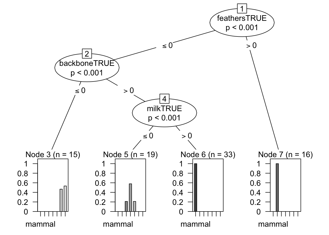

C 4.5 Decision Tree

C45Fit <- Zoo_train |> train(type ~ .,
  method = "J48",
  data = _,
    tuneLength = 5,
    trControl = trainControl(method = "cv", indexOut = train_index))
C45Fit

C4.5-like Trees 

83 samples
16 predictors
 7 classes: 'mammal', 'bird', 'reptile', 'fish', 'amphibian', 'insect', 'mollusc.et.al' 

No pre-processing
Resampling: Cross-Validated (10 fold) 
Summary of sample sizes: 76, 75, 73, 76, 74, 74, ... 
Resampling results across tuning parameters:

  C      M  Accuracy  Kappa
  0.010  1  0.975     0.967
  0.010  2  0.965     0.954
  0.010  3  0.953     0.940
  0.010  4  0.959     0.948
  0.010  5  0.970     0.962
  0.133  1  1.000     1.000
  0.133  2  0.976     0.968
  0.133  3  0.965     0.954
  0.133  4  0.959     0.948
  0.133  5  0.970     0.962
  0.255  1  1.000     1.000
  0.255  2  0.976     0.968
  0.255  3  0.965     0.954
  0.255  4  0.959     0.948
  0.255  5  0.970     0.962
  0.378  1  1.000     1.000
  0.378  2  0.976     0.968
  0.378  3  0.965     0.954
  0.378  4  0.959     0.948
  0.378  5  0.970     0.962
  0.500  1  1.000     1.000
  0.500  2  0.976     0.968
  0.500  3  0.965     0.954
  0.500  4  0.959     0.948
  0.500  5  0.970     0.962

Accuracy was used to select the optimal model using the largest value.
The final values used for the model were C = 0.133 and M = 1.

C45Fit$finalModel

J48 pruned tree
------------------

feathersTRUE <= 0
|   milkTRUE <= 0
|   |   backboneTRUE <= 0
|   |   |   predatorTRUE <= 0
|   |   |   |   legs <= 2: mollusc.et.al (1.0)
|   |   |   |   legs > 2: insect (6.0)
|   |   |   predatorTRUE > 0: mollusc.et.al (8.0/1.0)
|   |   backboneTRUE > 0
|   |   |   finsTRUE <= 0
|   |   |   |   aquaticTRUE <= 0: reptile (3.0)
|   |   |   |   aquaticTRUE > 0
|   |   |   |   |   eggsTRUE <= 0: reptile (1.0)
|   |   |   |   |   eggsTRUE > 0: amphibian (4.0)
|   |   |   finsTRUE > 0: fish (11.0)
|   milkTRUE > 0: mammal (33.0)
feathersTRUE > 0: bird (16.0)

Number of Leaves  :     9

Size of the tree :  17

K-Nearest Neighbors

Note: kNN uses Euclidean distance, so data should be standardized (scaled) first. Here legs are measured between 0 and 6 while all other variables are between 0 and 1. Scaling can be directly performed as preprocessing in train using the parameter preProcess = "scale".

knnFit <- Zoo_train |> train(type ~ .,
  method = "knn",
  data = _,
  preProcess = "scale",
    tuneLength = 5,
  tuneGrid=data.frame(k = 1:10),
    trControl = trainControl(method = "cv", indexOut = train_index))
knnFit

k-Nearest Neighbors 

83 samples
16 predictors
 7 classes: 'mammal', 'bird', 'reptile', 'fish', 'amphibian', 'insect', 'mollusc.et.al' 

Pre-processing: scaled (16) 
Resampling: Cross-Validated (10 fold) 
Summary of sample sizes: 77, 74, 75, 75, 74, 74, ... 
Resampling results across tuning parameters:

  k   Accuracy  Kappa
   1  1.000     1.000
   2  0.965     0.954
   3  0.963     0.951
   4  0.942     0.925
   5  0.941     0.921
   6  0.963     0.951
   7  0.963     0.951
   8  0.941     0.921
   9  0.908     0.883
  10  0.918     0.892

Accuracy was used to select the optimal model using the largest value.
The final value used for the model was k = 1.

knnFit$finalModel

1-nearest neighbor model
Training set outcome distribution:

       mammal          bird       reptile          fish     amphibian 
           33            16             4            11             4 
       insect mollusc.et.al 
            7             8

PART (Rule-based classifier)

rulesFit <- Zoo_train |> train(type ~ .,
  method = "PART",
  data = _,
  tuneLength = 5,
  trControl = trainControl(method = "cv", indexOut = train_index))
rulesFit

Rule-Based Classifier 

83 samples
16 predictors
 7 classes: 'mammal', 'bird', 'reptile', 'fish', 'amphibian', 'insect', 'mollusc.et.al' 

No pre-processing
Resampling: Cross-Validated (10 fold) 
Summary of sample sizes: 73, 74, 76, 76, 75, 74, ... 
Resampling results across tuning parameters:

  threshold  pruned  Accuracy  Kappa
  0.010      yes     0.979     0.973
  0.010      no      0.979     0.973
  0.133      yes     0.990     0.987
  0.133      no      0.979     0.973
  0.255      yes     0.990     0.987
  0.255      no      0.979     0.973
  0.378      yes     0.990     0.987
  0.378      no      0.979     0.973
  0.500      yes     0.990     0.987
  0.500      no      0.979     0.973

Accuracy was used to select the optimal model using the largest value.
The final values used for the model were threshold = 0.5 and pruned = yes.

rulesFit$finalModel

PART decision list
------------------

feathersTRUE <= 0 AND
milkTRUE > 0: mammal (33.0)

feathersTRUE > 0: bird (16.0)

backboneTRUE <= 0 AND
airborneTRUE <= 0 AND
predatorTRUE > 0: mollusc.et.al (7.0)

backboneTRUE > 0 AND
finsTRUE > 0: fish (11.0)

backboneTRUE <= 0: insect (8.0/1.0)

aquaticTRUE > 0: amphibian (5.0/1.0)

: reptile (3.0)

Number of Rules  :  7

Linear Support Vector Machines

svmFit <- Zoo_train |> train(type ~.,
  method = "svmLinear",
  data = _,
    tuneLength = 5,
    trControl = trainControl(method = "cv", indexOut = train_index))
svmFit

Support Vector Machines with Linear Kernel 

83 samples
16 predictors
 7 classes: 'mammal', 'bird', 'reptile', 'fish', 'amphibian', 'insect', 'mollusc.et.al' 

No pre-processing
Resampling: Cross-Validated (10 fold) 
Summary of sample sizes: 74, 74, 77, 75, 74, 77, ... 
Resampling results:

  Accuracy  Kappa
  1         1    

Tuning parameter 'C' was held constant at a value of 1

svmFit$finalModel

Support Vector Machine object of class "ksvm" 

SV type: C-svc  (classification) 
 parameter : cost C = 1 

Linear (vanilla) kernel function. 

Number of Support Vectors : 39 

Objective Function Value : -0.143 -0.217 -0.15 -0.175 -0.0934 -0.0974 -0.292 -0.0835 -0.154 -0.0901 -0.112 -0.189 -0.593 -0.13 -0.179 -0.122 -0.0481 -0.0838 -0.125 -0.15 -0.501 
Training error : 0

Random Forest

randomForestFit <- Zoo_train |> train(type ~ .,
  method = "rf",
  data = _,
    tuneLength = 5,
    trControl = trainControl(method = "cv", indexOut = train_index))
randomForestFit

Random Forest 

83 samples
16 predictors
 7 classes: 'mammal', 'bird', 'reptile', 'fish', 'amphibian', 'insect', 'mollusc.et.al' 

No pre-processing
Resampling: Cross-Validated (10 fold) 
Summary of sample sizes: 75, 76, 75, 76, 74, 73, ... 
Resampling results across tuning parameters:

  mtry  Accuracy  Kappa
   2    1         1    
   5    1         1    
   9    1         1    
  12    1         1    
  16    1         1    

Accuracy was used to select the optimal model using the largest value.
The final value used for the model was mtry = 2.

randomForestFit$finalModel


Call:
 randomForest(x = x, y = y, mtry = param$mtry) 
               Type of random forest: classification
                     Number of trees: 500
No. of variables tried at each split: 2

        OOB estimate of  error rate: 7.23%
Confusion matrix:
              mammal bird reptile fish amphibian insect mollusc.et.al
mammal            33    0       0    0         0      0             0
bird               0   16       0    0         0      0             0
reptile            0    1       0    2         1      0             0
fish               0    0       0   11         0      0             0
amphibian          0    0       0    0         4      0             0
insect             0    0       0    0         0      7             0
mollusc.et.al      1    0       0    0         0      1             6
              class.error
mammal               0.00
bird                 0.00
reptile              1.00
fish                 0.00
amphibian            0.00
insect               0.00
mollusc.et.al        0.25

Gradient Boosted Decision Trees (xgboost)

xgboostFit <- Zoo_train |> train(type ~ .,
  method = "xgbTree",
  data = _,
  tuneLength = 5,
  trControl = trainControl(method = "cv", indexOut = train_index),
  tuneGrid = expand.grid(
    nrounds = 20,
    max_depth = 3,
    colsample_bytree = .6,
    eta = 0.1,
    gamma=0,
    min_child_weight = 1,
    subsample = .5
  ))
xgboostFit

eXtreme Gradient Boosting 

83 samples
16 predictors
 7 classes: 'mammal', 'bird', 'reptile', 'fish', 'amphibian', 'insect', 'mollusc.et.al' 

No pre-processing
Resampling: Cross-Validated (10 fold) 
Summary of sample sizes: 77, 73, 74, 75, 75, 75, ... 
Resampling results:

  Accuracy  Kappa
  0.973     0.964

Tuning parameter 'nrounds' was held constant at a value of 20
Tuning
 held constant at a value of 1
Tuning parameter 'subsample' was held
 constant at a value of 0.5

xgboostFit$finalModel

##### xgb.Booster
raw: 112.4 Kb 
call:
  xgboost::xgb.train(params = list(eta = param$eta, max_depth = param$max_depth, 
    gamma = param$gamma, colsample_bytree = param$colsample_bytree, 
    min_child_weight = param$min_child_weight, subsample = param$subsample), 
    data = x, nrounds = param$nrounds, num_class = length(lev), 
    objective = "multi:softprob")
params (as set within xgb.train):
  eta = "0.1", max_depth = "3", gamma = "0", colsample_bytree = "0.6", min_child_weight = "1", subsample = "0.5", num_class = "7", objective = "multi:softprob", validate_parameters = "TRUE"
xgb.attributes:
  niter
callbacks:
  cb.print.evaluation(period = print_every_n)
# of features: 16 
niter: 20
nfeatures : 16 
xNames : hairTRUE feathersTRUE eggsTRUE milkTRUE airborneTRUE aquaticTRUE predatorTRUE toothedTRUE backboneTRUE breathesTRUE venomousTRUE finsTRUE legs tailTRUE domesticTRUE catsizeTRUE 
problemType : Classification 
tuneValue :
      nrounds max_depth eta gamma colsample_bytree min_child_weight subsample
1      20         3 0.1     0              0.6                1       0.5
obsLevels : mammal bird reptile fish amphibian insect mollusc.et.al 
param :
    list()

Artificial Neural Network

nnetFit <- Zoo_train |> train(type ~ .,
  method = "nnet",
  data = _,
    tuneLength = 5,
    trControl = trainControl(method = "cv", indexOut = train_index),
  trace = FALSE)
nnetFit

Neural Network 

83 samples
16 predictors
 7 classes: 'mammal', 'bird', 'reptile', 'fish', 'amphibian', 'insect', 'mollusc.et.al' 

No pre-processing
Resampling: Cross-Validated (10 fold) 
Summary of sample sizes: 75, 74, 74, 74, 74, 75, ... 
Resampling results across tuning parameters:

  size  decay  Accuracy  Kappa
  1     0e+00  0.776     0.681
  1     1e-04  0.789     0.709
  1     1e-03  0.911     0.882
  1     1e-02  0.832     0.781
  1     1e-01  0.722     0.621
  3     0e+00  0.963     0.950
  3     1e-04  0.976     0.968
  3     1e-03  0.986     0.979
  3     1e-02  0.986     0.981
  3     1e-01  0.976     0.968
  5     0e+00  0.965     0.953
  5     1e-04  0.986     0.981
  5     1e-03  0.986     0.981
  5     1e-02  0.986     0.981
  5     1e-01  0.986     0.981
  7     0e+00  0.976     0.968
  7     1e-04  0.986     0.981
  7     1e-03  0.986     0.981
  7     1e-02  0.986     0.981
  7     1e-01  0.986     0.981
  9     0e+00  0.986     0.981
  9     1e-04  0.986     0.981
  9     1e-03  0.986     0.981
  9     1e-02  0.986     0.981
  9     1e-01  0.986     0.981

Accuracy was used to select the optimal model using the largest value.
The final values used for the model were size = 3 and decay = 0.01.

nnetFit$finalModel

a 16-3-7 network with 79 weights
inputs: hairTRUE feathersTRUE eggsTRUE milkTRUE airborneTRUE aquaticTRUE predatorTRUE toothedTRUE backboneTRUE breathesTRUE venomousTRUE finsTRUE legs tailTRUE domesticTRUE catsizeTRUE 
output(s): .outcome 
options were - softmax modelling  decay=0.01

Comparing Models

Collect the performance metrics from the models trained on the same data.

resamps <- resamples(list(
  ctree = ctreeFit,
  C45 = C45Fit,
  SVM = svmFit,
  KNN = knnFit,
  rules = rulesFit,
  randomForest = randomForestFit,
  xgboost = xgboostFit,
  NeuralNet = nnetFit
    ))
resamps


Call:
resamples.default(x = list(ctree = ctreeFit, C45 = C45Fit, SVM = svmFit, KNN
 = knnFit, rules = rulesFit, randomForest = randomForestFit, xgboost
 = xgboostFit, NeuralNet = nnetFit))

Models: ctree, C45, SVM, KNN, rules, randomForest, xgboost, NeuralNet 
Number of resamples: 10 
Performance metrics: Accuracy, Kappa 
Time estimates for: everything, final model fit

Calculate summary statistics

summary(resamps)


Call:
summary.resamples(object = resamps)

Models: ctree, C45, SVM, KNN, rules, randomForest, xgboost, NeuralNet 
Number of resamples: 10 

Accuracy 
              Min. 1st Qu. Median  Mean 3rd Qu. Max. NA's
ctree        0.700   0.778  0.817 0.827   0.871    1    0
C45          1.000   1.000  1.000 1.000   1.000    1    0
SVM          1.000   1.000  1.000 1.000   1.000    1    0
KNN          1.000   1.000  1.000 1.000   1.000    1    0
rules        0.900   1.000  1.000 0.990   1.000    1    0
randomForest 1.000   1.000  1.000 1.000   1.000    1    0
xgboost      0.857   1.000  1.000 0.973   1.000    1    0
NeuralNet    0.857   1.000  1.000 0.986   1.000    1    0

Kappa 
              Min. 1st Qu. Median  Mean 3rd Qu. Max. NA's
ctree        0.634   0.715  0.748 0.772   0.815    1    0
C45          1.000   1.000  1.000 1.000   1.000    1    0
SVM          1.000   1.000  1.000 1.000   1.000    1    0
KNN          1.000   1.000  1.000 1.000   1.000    1    0
rules        0.868   1.000  1.000 0.987   1.000    1    0
randomForest 1.000   1.000  1.000 1.000   1.000    1    0
xgboost      0.806   1.000  1.000 0.964   1.000    1    0
NeuralNet    0.806   1.000  1.000 0.981   1.000    1    0

library(lattice)
bwplot(resamps, layout = c(3, 1))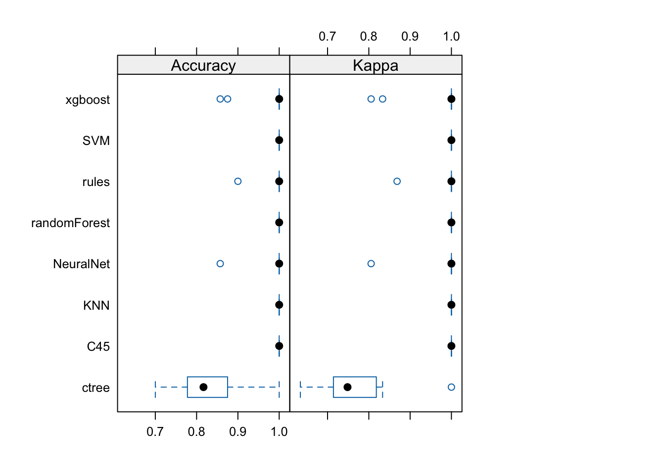

Perform inference about differences between models. For each metric, all pair-wise differences are computed and tested to assess if the difference is equal to zero. By default Bonferroni correction for multiple comparison is used. Differences are shown in the upper triangle and p-values are in the lower triangle.

difs <- diff(resamps)
difs


Call:
diff.resamples(x = resamps)

Models: ctree, C45, SVM, KNN, rules, randomForest, xgboost, NeuralNet 
Metrics: Accuracy, Kappa 
Number of differences: 28 
p-value adjustment: bonferroni

summary(difs)


Call:
summary.diff.resamples(object = difs)

p-value adjustment: bonferroni 
Upper diagonal: estimates of the difference
Lower diagonal: p-value for H0: difference = 0

Accuracy 
             ctree   C45      SVM      KNN      rules    randomForest xgboost 
ctree                -0.17262 -0.17262 -0.17262 -0.16262 -0.17262     -0.14583
C45          0.00193           0.00000  0.00000  0.01000  0.00000      0.02679
SVM          0.00193 NA                 0.00000  0.01000  0.00000      0.02679
KNN          0.00193 NA       NA                 0.01000  0.00000      0.02679
rules        0.00376 1.00000  1.00000  1.00000           -0.01000      0.01679
randomForest 0.00193 NA       NA       NA       1.00000                0.02679
xgboost      0.05129 1.00000  1.00000  1.00000  1.00000  1.00000              
NeuralNet    0.01405 1.00000  1.00000  1.00000  1.00000  1.00000      1.00000 
             NeuralNet
ctree        -0.15833 
C45           0.01429 
SVM           0.01429 
KNN           0.01429 
rules         0.00429 
randomForest  0.01429 
xgboost      -0.01250 
NeuralNet             

Kappa 
             ctree   C45      SVM      KNN      rules    randomForest xgboost 
ctree                -0.22840 -0.22840 -0.22840 -0.21524 -0.22840     -0.19229
C45          0.00116           0.00000  0.00000  0.01316  0.00000      0.03611
SVM          0.00116 NA                 0.00000  0.01316  0.00000      0.03611
KNN          0.00116 NA       NA                 0.01316  0.00000      0.03611
rules        0.00238 1.00000  1.00000  1.00000           -0.01316      0.02295
randomForest 0.00116 NA       NA       NA       1.00000                0.03611
xgboost      0.04216 1.00000  1.00000  1.00000  1.00000  1.00000              
NeuralNet    0.01055 1.00000  1.00000  1.00000  1.00000  1.00000      1.00000 
             NeuralNet
ctree        -0.20895 
C45           0.01944 
SVM           0.01944 
KNN           0.01944 
rules         0.00629 
randomForest  0.01944 
xgboost      -0.01667 
NeuralNet

All perform similarly well except ctree (differences in the first row are negative and the p-values in the first column are <.05 indicating that the null-hypothesis of a difference of 0 can be rejected).

Applying the Chosen Model to the Test Data

Most models do similarly well on the data. We choose here the random forest model.

pr <- predict(randomForestFit, Zoo_test)
pr

 [1] mammal        mammal        mammal        fish          fish         
 [6] bird          bird          mammal        mammal        mammal       
[11] mammal        mollusc.et.al reptile       mammal        bird         
[16] mollusc.et.al bird          insect       
Levels: mammal bird reptile fish amphibian insect mollusc.et.al

Calculate the confusion matrix for the held-out test data.

confusionMatrix(pr, reference = Zoo_test$type)

Confusion Matrix and Statistics

               Reference
Prediction      mammal bird reptile fish amphibian insect mollusc.et.al
  mammal             8    0       0    0         0      0             0
  bird               0    4       0    0         0      0             0
  reptile            0    0       1    0         0      0             0
  fish               0    0       0    2         0      0             0
  amphibian          0    0       0    0         0      0             0
  insect             0    0       0    0         0      1             0
  mollusc.et.al      0    0       0    0         0      0             2

Overall Statistics
                                    
               Accuracy : 1         
                 95% CI : (0.815, 1)
    No Information Rate : 0.444     
    P-Value [Acc > NIR] : 4.58e-07  
                                    
                  Kappa : 1         
                                    
 Mcnemar's Test P-Value : NA        

Statistics by Class:

                     Class: mammal Class: bird Class: reptile Class: fish
Sensitivity                  1.000       1.000         1.0000       1.000
Specificity                  1.000       1.000         1.0000       1.000
Pos Pred Value               1.000       1.000         1.0000       1.000
Neg Pred Value               1.000       1.000         1.0000       1.000
Prevalence                   0.444       0.222         0.0556       0.111
Detection Rate               0.444       0.222         0.0556       0.111
Detection Prevalence         0.444       0.222         0.0556       0.111
Balanced Accuracy            1.000       1.000         1.0000       1.000
                     Class: amphibian Class: insect Class: mollusc.et.al
Sensitivity                        NA        1.0000                1.000
Specificity                         1        1.0000                1.000
Pos Pred Value                     NA        1.0000                1.000
Neg Pred Value                     NA        1.0000                1.000
Prevalence                          0        0.0556                0.111
Detection Rate                      0        0.0556                0.111
Detection Prevalence                0        0.0556                0.111
Balanced Accuracy                  NA        1.0000                1.000

Comparing Decision Boundaries of Popular Classification Techniques

Classifiers create decision boundaries to discriminate between classes. Different classifiers are able to create different shapes of decision boundaries (e.g., some are strictly linear) and thus some classifiers may perform better for certain datasets. This page visualizes the decision boundaries found by several popular classification methods.

The following plot adds the decision boundary (black lines) and classification confidence (color intensity) by evaluating the classifier at evenly spaced grid points. Note that low resolution (to make evaluation faster) will make the decision boundary look like it has small steps even if it is a (straight) line.

library(scales)
library(tidyverse)
library(ggplot2)
library(caret)

decisionplot <- function(model, data, class_var, 
  predict_type = c("class", "prob"), resolution = 3 * 72) {
  # resolution is set to 72 dpi if the image is rendered  3 inches wide. 
  
  y <- data |> pull(class_var)
  x <- data |> dplyr::select(-all_of(class_var))
  
  # resubstitution accuracy
  prediction <- predict(model, x, type = predict_type[1])
  # LDA returns a list
  if(is.list(prediction)) prediction <- prediction$class
  prediction <- factor(prediction, levels = levels(y))
  
  cm <- confusionMatrix(data = prediction, 
                        reference = y)
  acc <- cm$overall["Accuracy"]
  
  # evaluate model on a grid
  r <- sapply(x[, 1:2], range, na.rm = TRUE)
  xs <- seq(r[1,1], r[2,1], length.out = resolution)
  ys <- seq(r[1,2], r[2,2], length.out = resolution)
  g <- cbind(rep(xs, each = resolution), rep(ys, time = resolution))
  colnames(g) <- colnames(r)
  g <- as_tibble(g)
  
  ### guess how to get class labels from predict
  ### (unfortunately not very consistent between models)
  cl <- predict(model, g, type = predict_type[1])
  
  # LDA returns a list
  prob <- NULL
  if(is.list(cl)) { 
    prob <- cl$posterior
    cl <- cl$class
  } else
    if(!is.na(predict_type[2]))
      try(prob <- predict(model, g, type = predict_type[2]))
  
  # we visualize the difference in probability/score between the 
  # winning class and the second best class.
  # don't use probability if predict for the classifier does not support it.
  max_prob <- 1
  if(!is.null(prob))
    try({
      max_prob <- t(apply(prob, MARGIN = 1, sort, decreasing = TRUE))
      max_prob <- max_prob[,1] - max_prob[,2]
    }, silent = TRUE) 
  
  cl <- factor(cl, levels = levels(y))
  
  g <- g |> add_column(prediction = cl, probability = max_prob)
  
  ggplot(g, mapping = aes(
    x = .data[[colnames(g)[1]]], y = .data[[colnames(g)[2]]])) +
    geom_raster(mapping = aes(fill = prediction, alpha = probability)) +
    geom_contour(mapping = aes(z = as.numeric(prediction)), 
      bins = length(levels(cl)), linewidth = .5, color = "black") +
    geom_point(data = data, mapping =  aes(
      x = .data[[colnames(data)[1]]], 
      y = .data[[colnames(data)[2]]],
      shape = .data[[class_var]]), alpha = .7) + 
    scale_alpha_continuous(range = c(0,1), limits = c(0,1), guide = "none") +  
    labs(subtitle = paste("Training accuracy:", round(acc, 2))) +
     theme_minimal(base_size = 14)
}

Penguins Dataset

For easier visualization, we use two dimensions of the penguins dataset. Contour lines visualize the density like mountains on a map.

set.seed(1000)
data("penguins")
penguins <- as_tibble(penguins) |>
  drop_na()

### Three classes 
### (note: MASS also has a select function which hides dplyr's select)
x <- penguins |> dplyr::select(bill_length_mm, bill_depth_mm, species)
x

# A tibble: 333 × 3
   bill_length_mm bill_depth_mm species
            <dbl>         <dbl> <fct>  
 1           39.1          18.7 Adelie 
 2           39.5          17.4 Adelie 
 3           40.3          18   Adelie 
 4           36.7          19.3 Adelie 
 5           39.3          20.6 Adelie 
 6           38.9          17.8 Adelie 
 7           39.2          19.6 Adelie 
 8           41.1          17.6 Adelie 
 9           38.6          21.2 Adelie 
10           34.6          21.1 Adelie 
# ℹ 323 more rows

ggplot(x, aes(x = bill_length_mm, y = bill_depth_mm, fill = species)) +  
  stat_density_2d(geom = "polygon", aes(alpha = after_stat(level))) +
  geom_point() +
  theme_minimal(base_size = 14) +
  labs(x = "Bill length (mm)",
       y = "Bill depth (mm)",
       fill = "Species",
       alpha = "Density")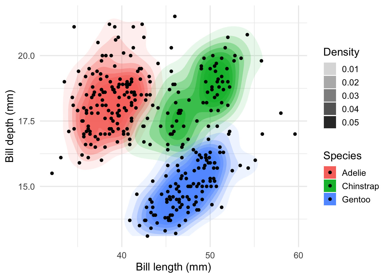

Note: There is some overplotting and you could use geom_jitter() instead of geom_point().

K-Nearest Neighbors Classifier

model <- x |> caret::knn3(species ~ ., data = _, k = 1)
decisionplot(model, x, class_var = "species") + 
  labs(title = "kNN (1 neighbor)",
       x = "Bill length (mm)",
       y = "Bill depth (mm)",
       shape = "Species",
       fill = "Prediction")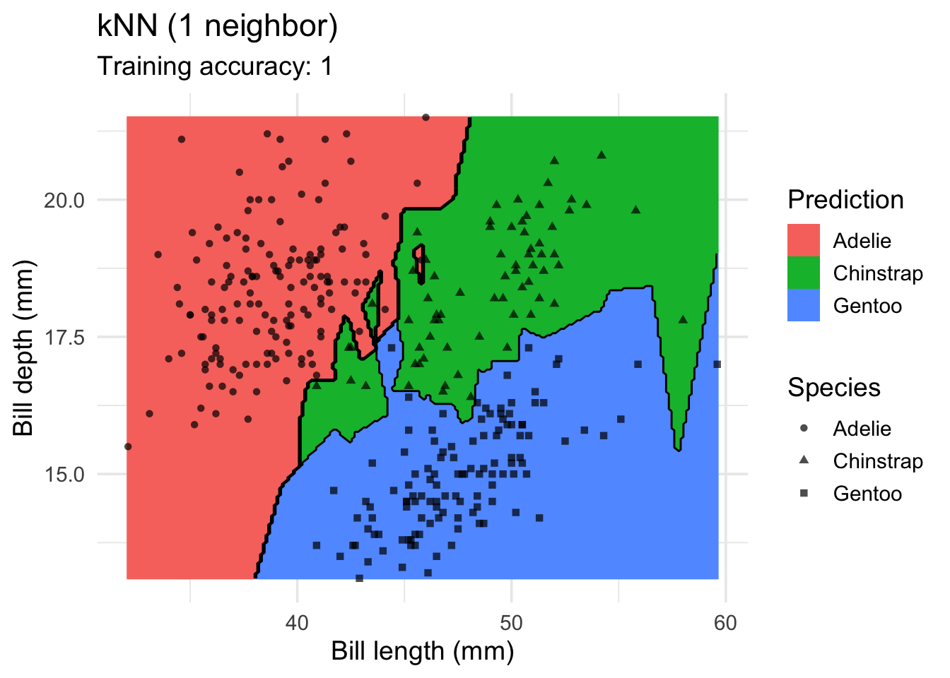

model <- x |> caret::knn3(species ~ ., data = _, k = 3)
decisionplot(model, x, class_var = "species") + 
  labs(title = "kNN (3 neighbor)",
       x = "Bill length (mm)",
       y = "Bill depth (mm)",
       shape = "Species",
       fill = "Prediction")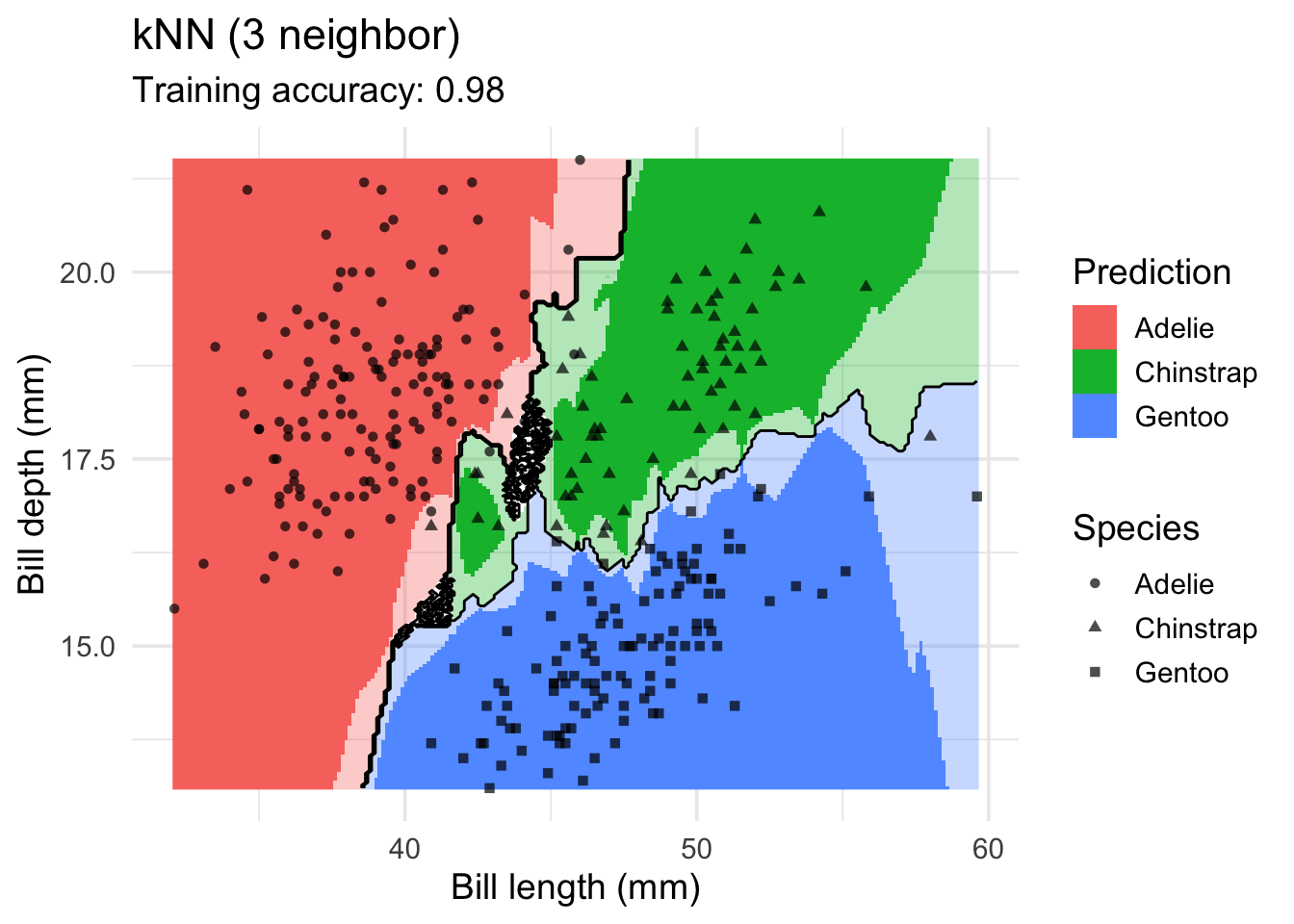

model <- x |> caret::knn3(species ~ ., data = _, k = 9)
decisionplot(model, x, class_var = "species") + 
  labs(title = "kNN (9 neighbor)",
       x = "Bill length (mm)",
       y = "Bill depth (mm)",
       shape = "Species",
       fill = "Prediction")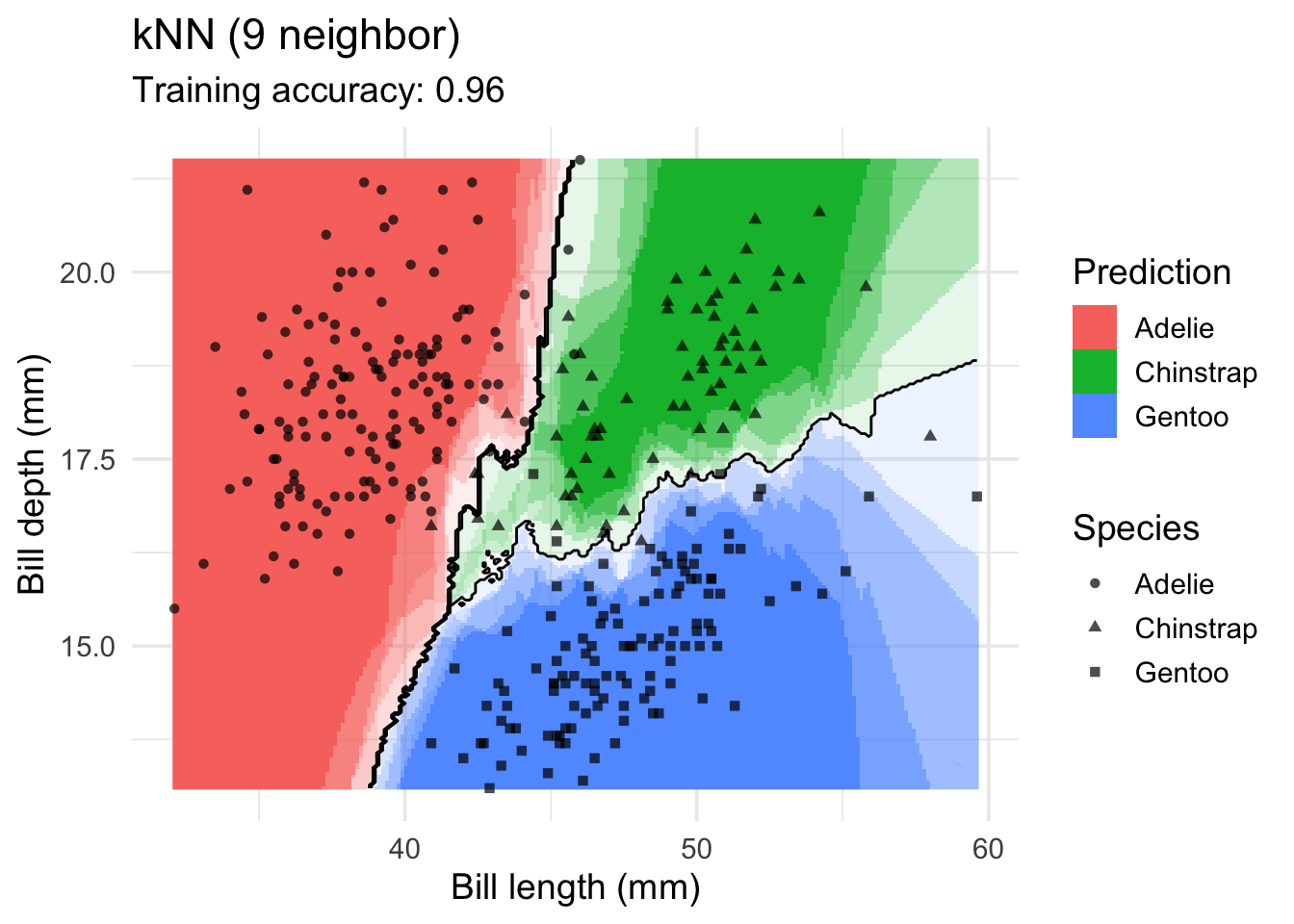

Increasing \(k\) smooths the decision boundary. At \(k=1\), we see white areas around points where penguins of two classes are in the same spot. Here, the algorithm randomly chooses a class during prediction resulting in the meandering decision boundary. The predictions in that area are not stable and every time we ask for a class, we may get a different class.

Naive Bayes Classifier

model <- x |> e1071::naiveBayes(species ~ ., data = _)
decisionplot(model, x, class_var = "species", 
             predict_type = c("class", "raw")) + 
  labs(title = "Naive Bayes",
       x = "Bill length (mm)",
       y = "Bill depth (mm)",
       shape = "Species",
       fill = "Prediction")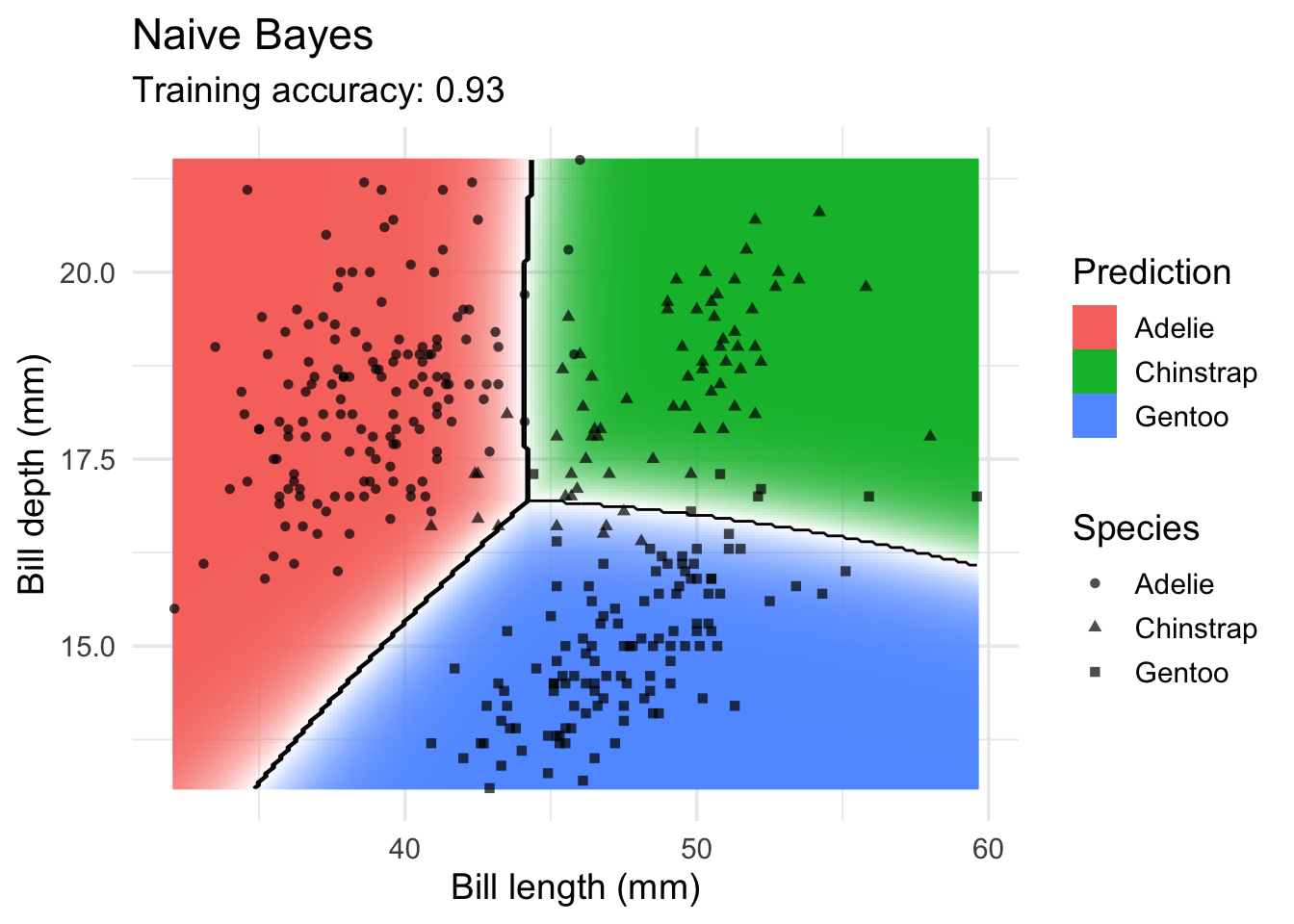

Linear Discriminant Analysis

model <- x |> MASS::lda(species ~ ., data = _)
decisionplot(model, x, class_var = "species") + 
  labs(title = "LDA",
       x = "Bill length (mm)",
       y = "Bill depth (mm)",
       shape = "Species",
       fill = "Prediction")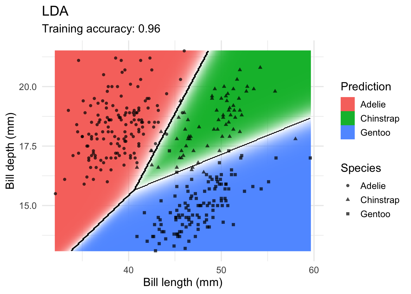

Multinomial Logistic Regression (implemented in nnet)

Multinomial logistic regression is an extension of logistic regression to problems with more than two classes.

model <- x |> nnet::multinom(species ~., data = _)

# weights:  12 (6 variable)
initial  value 365.837892 
iter  10 value 26.650783
iter  20 value 23.943597
iter  30 value 23.916873
iter  40 value 23.901339
iter  50 value 23.895442
iter  60 value 23.894251
final  value 23.892065 
converged

decisionplot(model, x, class_var = "species") + 
  labs(title = "Multinomial Logistic Regression",
       x = "Bill length (mm)",
       y = "Bill depth (mm)",
       shape = "Species",
       fill = "Prediction")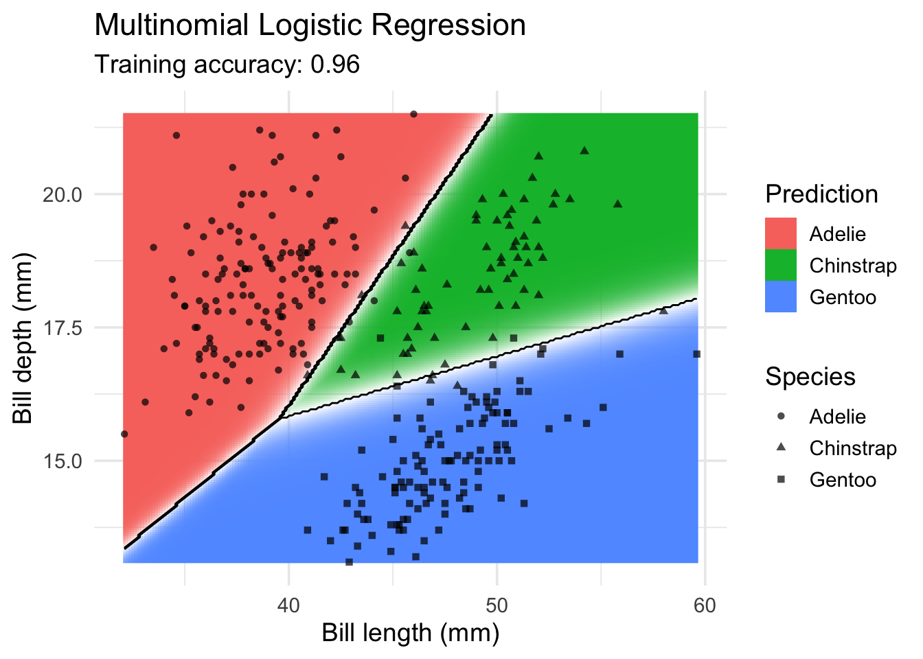

Decision Trees

model <- x |> rpart::rpart(species ~ ., data = _)
decisionplot(model, x, class_var = "species") + 
  labs(title = "CART",
       x = "Bill length (mm)",
       y = "Bill depth (mm)",
       shape = "Species",
       fill = "Prediction")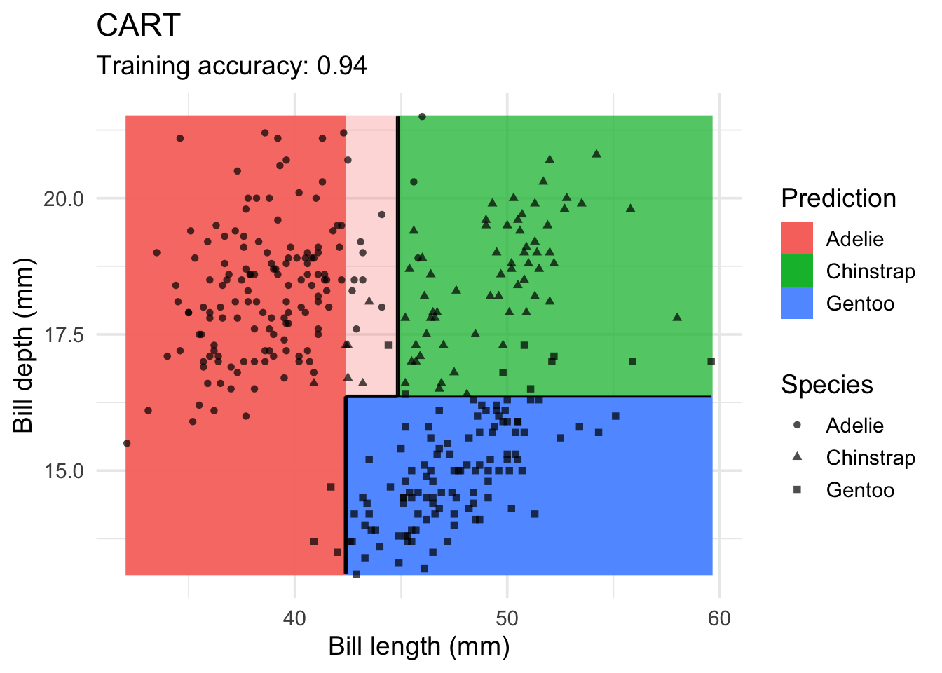

model <- x |> rpart::rpart(species ~ ., data = _,
  control = rpart.control(cp = 0.001, minsplit = 1))
decisionplot(model, x, class_var = "species") + 
  labs(title = "CART (overfitting)",
       x = "Bill length (mm)",
       y = "Bill depth (mm)",
       shape = "Species",
       fill = "Prediction")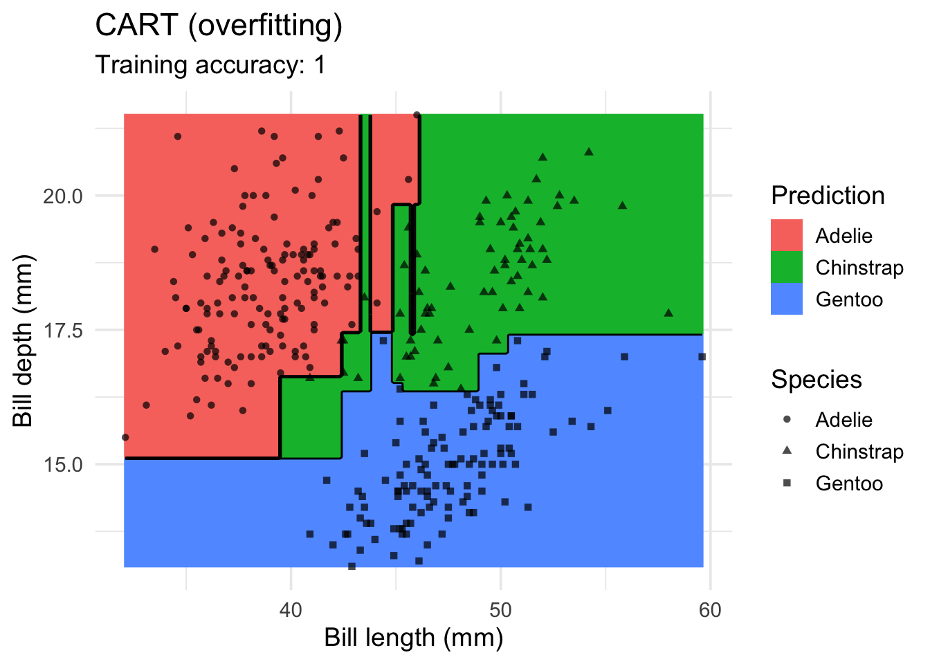

model <- x |> C50::C5.0(species ~ ., data = _)
decisionplot(model, x, class_var = "species") + 
  labs(title = "C5.0",
       x = "Bill length (mm)",
       y = "Bill depth (mm)",
       shape = "Species",
       fill = "Prediction")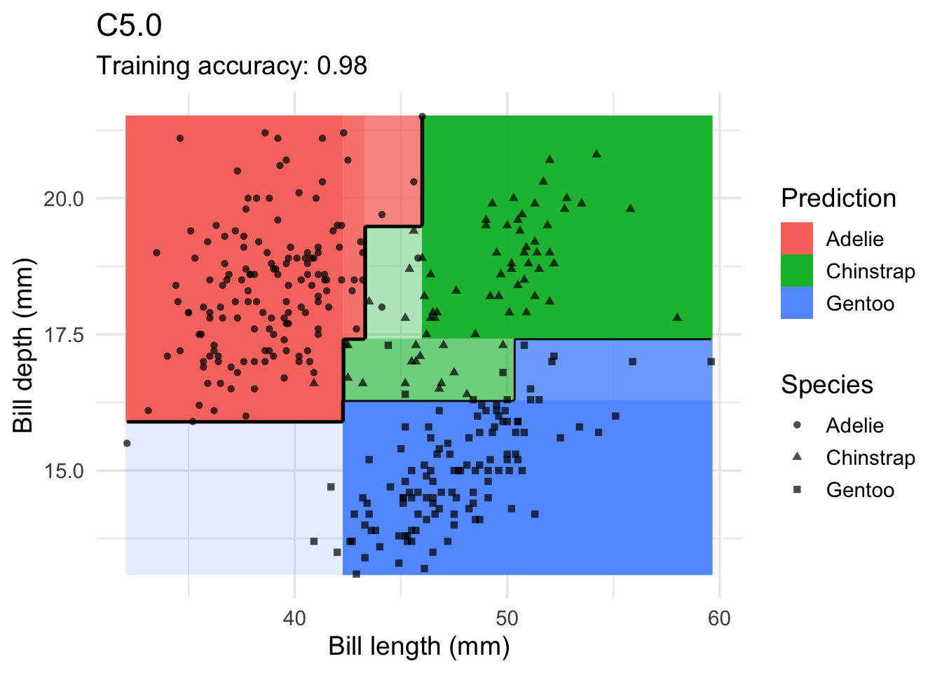

model <- x |> randomForest::randomForest(species ~ ., data = _)
decisionplot(model, x, class_var = "species") + 
  labs(title = "Random Forest",
       x = "Bill length (mm)",
       y = "Bill depth (mm)",
       shape = "Species",
       fill = "Prediction")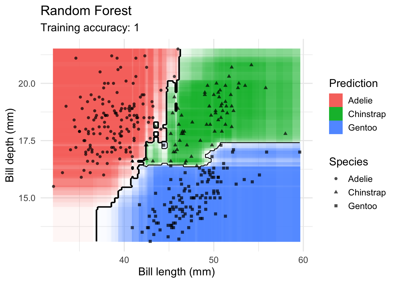

SVM

model <- x |> e1071::svm(species ~ ., data = _, kernel = "linear")
decisionplot(model, x, class_var = "species") + 
  labs(title = "SVM (linear kernel)",
       x = "Bill length (mm)",
       y = "Bill depth (mm)",
       shape = "Species",
       fill = "Prediction")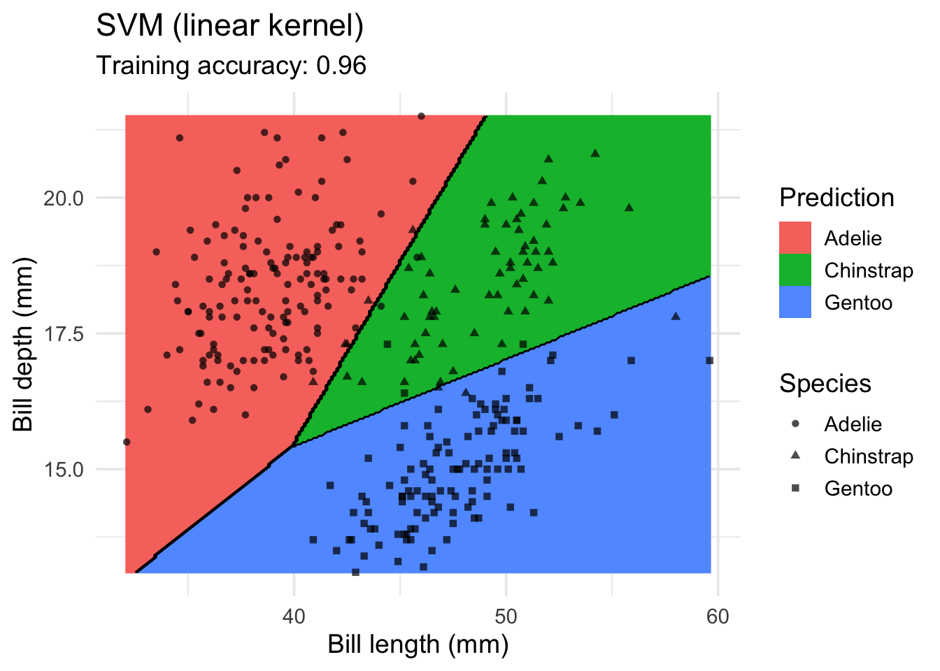

model <- x |> e1071::svm(species ~ ., data = _, kernel = "radial")
decisionplot(model, x, class_var = "species") + 
  labs(title = "SVM (radial kernel)",
       x = "Bill length (mm)",
       y = "Bill depth (mm)",
       shape = "Species",
       fill = "Prediction")

model <- x |> e1071::svm(species ~ ., data = _, kernel = "polynomial")
decisionplot(model, x, class_var = "species") + 
  labs(title = "SVM (polynomial kernel)",
       x = "Bill length (mm)",
       y = "Bill depth (mm)",
       shape = "Species",
       fill = "Prediction")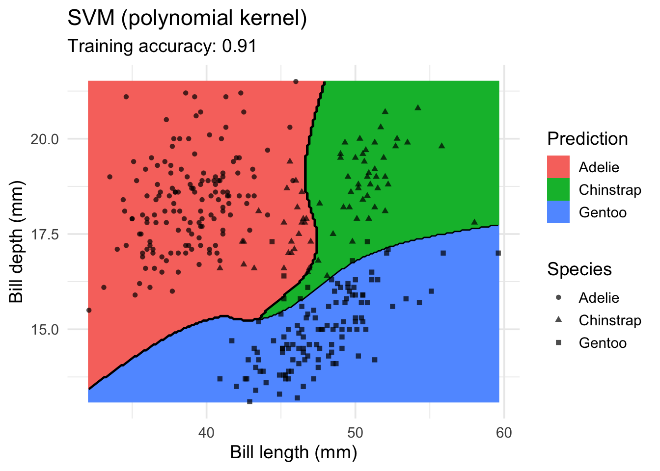

model <- x |> e1071::svm(species ~ ., data = _, kernel = "sigmoid")
decisionplot(model, x, class_var = "species") + 
  labs(title = "SVM (sigmoid kernel)",
       x = "Bill length (mm)",
       y = "Bill depth (mm)",
       shape = "Species",
       fill = "Prediction")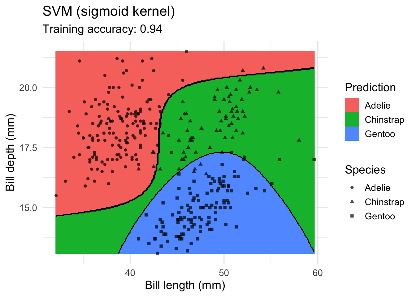

Single Layer Feed-forward Neural Networks

model <-x |> nnet::nnet(species ~ ., data = _, size = 1, trace = FALSE)
decisionplot(model, x, class_var  = "species", 
  predict_type = c("class", "raw")) + 
  labs(title = "NN (1 neuron)",
       x = "Bill length (mm)",
       y = "Bill depth (mm)",
       shape = "Species",
       fill = "Prediction")

Warning: Computation failed in `stat_contour()`
Caused by error in `if (zero_range(range)) ...`:
! missing value where TRUE/FALSE needed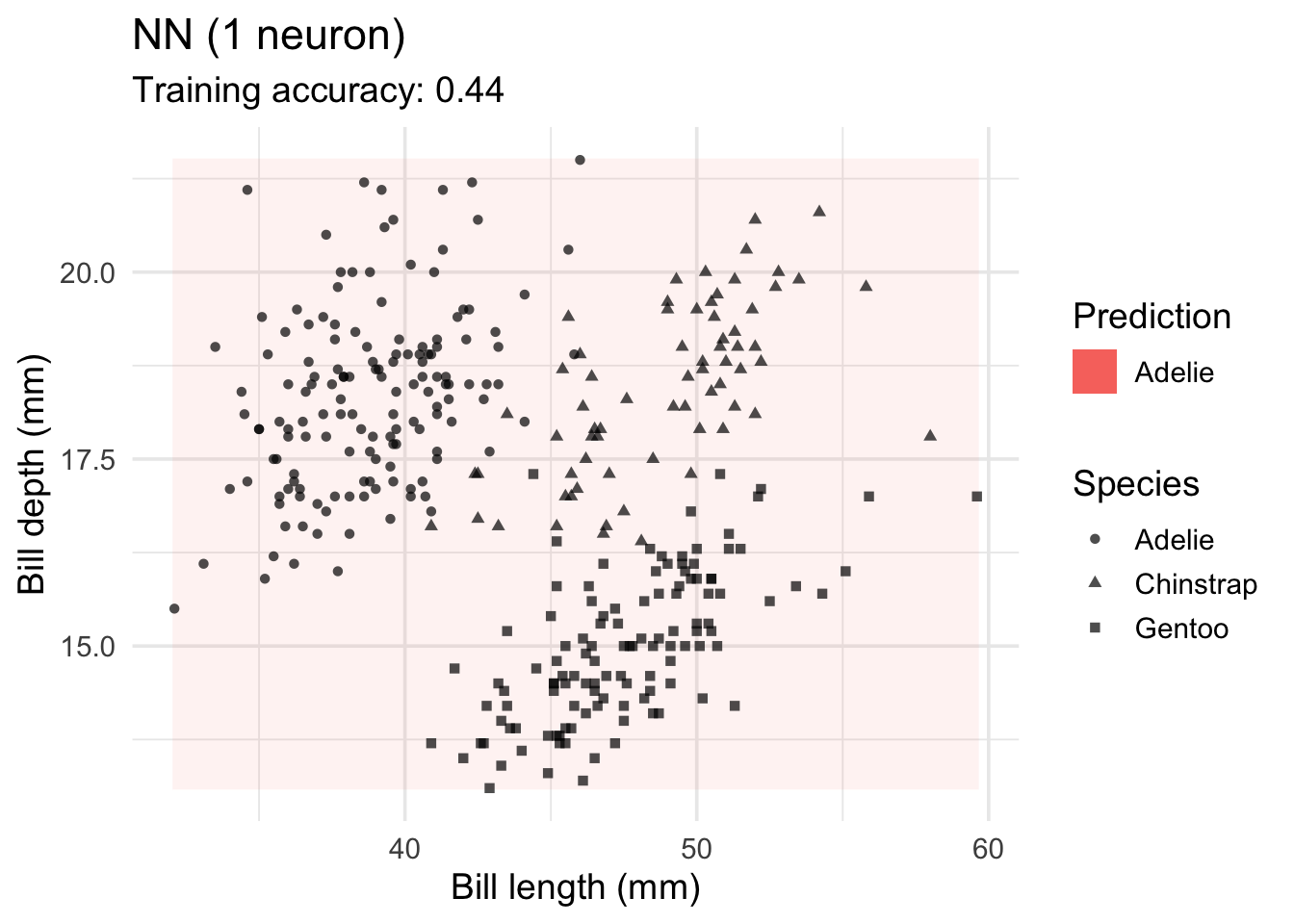

model <-x |> nnet::nnet(species ~ ., data = _, size = 2, trace = FALSE)
decisionplot(model, x, class_var  = "species", 
  predict_type = c("class", "raw")) + 
  labs(title = "NN (2 neurons)",
       x = "Bill length (mm)",
       y = "Bill depth (mm)",
       shape = "Species",
       fill = "Prediction")

Warning: Computation failed in `stat_contour()`
Caused by error in `if (zero_range(range)) ...`:
! missing value where TRUE/FALSE needed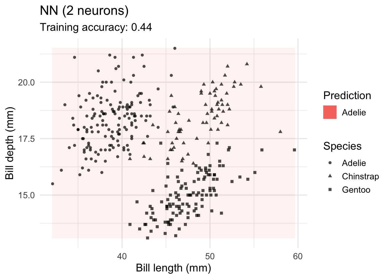

model <-x |> nnet::nnet(species ~ ., data = _, size = 4, trace = FALSE)
decisionplot(model, x, class_var  = "species", 
  predict_type = c("class", "raw")) + 
  labs(title = "NN (4 neurons)",
       x = "Bill length (mm)",
       y = "Bill depth (mm)",
       shape = "Species",
       fill = "Prediction")

model <-x |> nnet::nnet(species ~ ., data = _, size = 10, trace = FALSE)
decisionplot(model, x, class_var  = "species", 
  predict_type = c("class", "raw")) + 
  labs(title = "NN (10 neurons)",
       x = "Bill length (mm)",
       y = "Bill depth (mm)",
       shape = "Species",
       fill = "Prediction")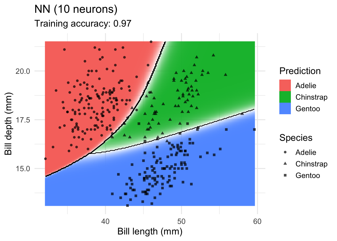

Circle Dataset

This set is not linearly separable!

set.seed(1000)

x <- mlbench::mlbench.circle(500)
###x <- mlbench::mlbench.cassini(500)
###x <- mlbench::mlbench.spirals(500, sd = .1)
###x <- mlbench::mlbench.smiley(500)
x <- cbind(as.data.frame(x$x), factor(x$classes))
colnames(x) <- c("x", "y", "class")
x <- as_tibble(x)
x

# A tibble: 500 × 3
         x       y class
     <dbl>   <dbl> <fct>
 1 -0.344   0.448  1    
 2  0.518   0.915  2    
 3 -0.772  -0.0913 1    
 4  0.382   0.412  1    
 5  0.0328  0.438  1    
 6 -0.865  -0.354  2    
 7  0.477   0.640  2    
 8  0.167  -0.809  2    
 9 -0.568  -0.281  1    
10 -0.488   0.638  2    
# ℹ 490 more rows

ggplot(x, aes(x = x, y = y, color = class)) + 
  geom_point() +
  theme_minimal(base_size = 14)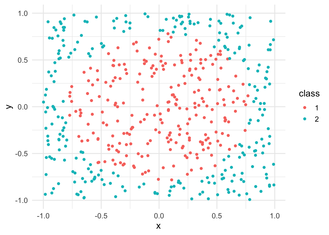

K-Nearest Neighbors Classifier

model <- x |> caret::knn3(class ~ ., data = _, k = 1)
decisionplot(model, x, class_var = "class") + 
  labs(title = "kNN (1 neighbor)",
       shape = "Class",
       fill = "Prediction")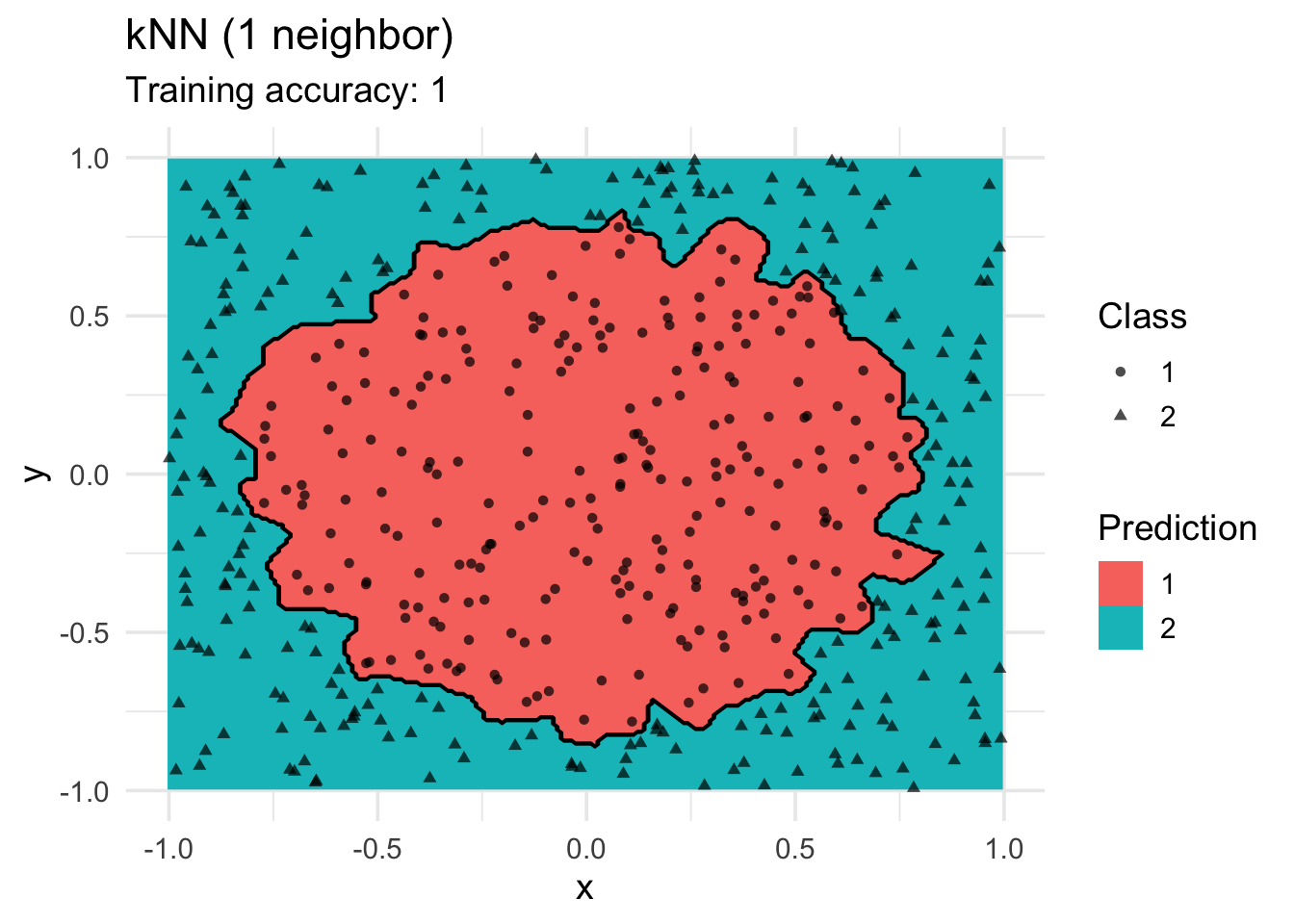

model <- x |> caret::knn3(class ~ ., data = _, k = 10)
decisionplot(model, x, class_var = "class") + 
  labs(title = "kNN (10 neighbor)",
       shape = "Class",
       fill = "Prediction")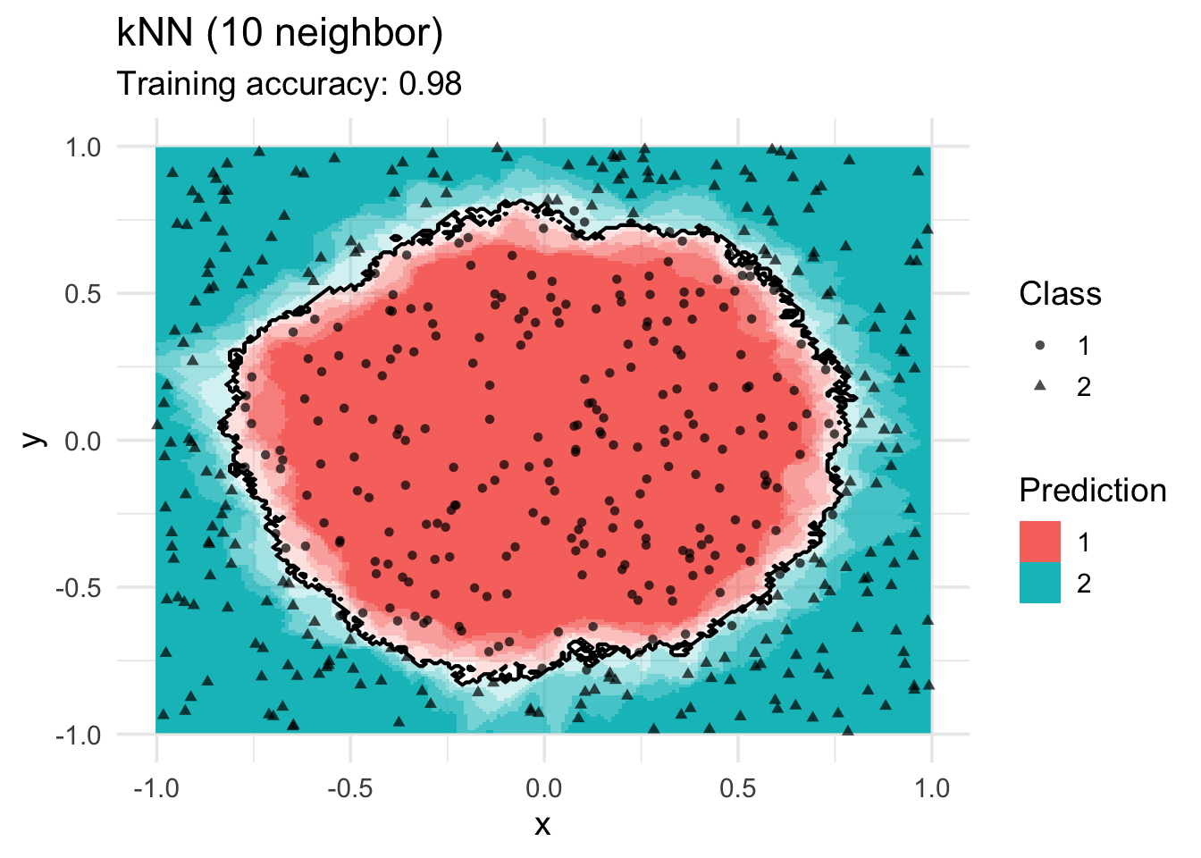

Naive Bayes Classifier

model <- x |> e1071::naiveBayes(class ~ ., data = _)
decisionplot(model, x, class_var = "class", 
  predict_type = c("class", "raw")) + 
  labs(title = "naive Bayes",
       shape = "Class",
       fill = "Prediction")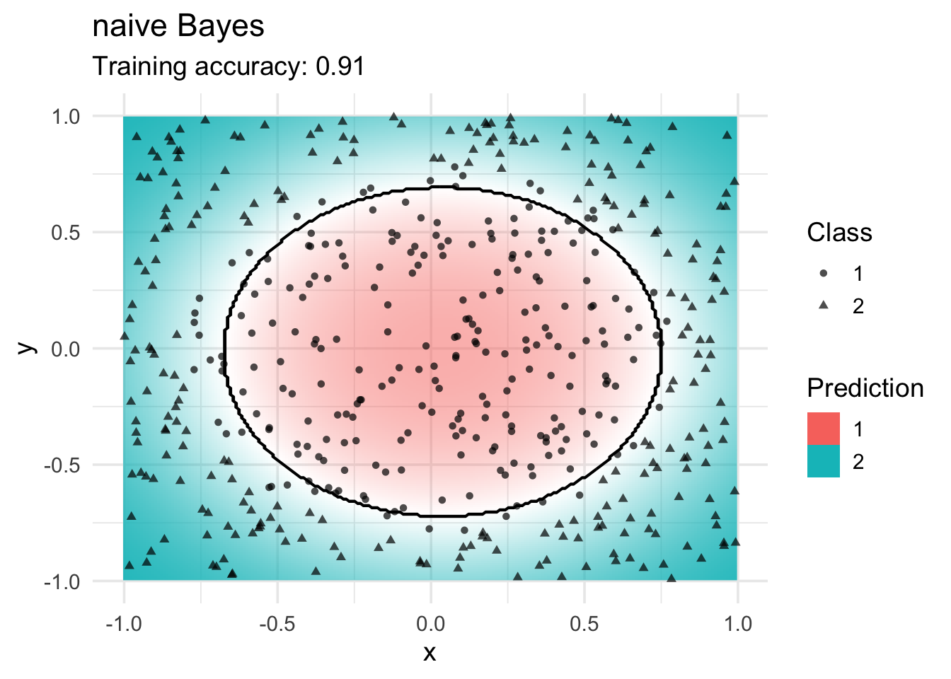

Linear Discriminant Analysis

LDA cannot find a good model since the true decision boundary is not linear.

model <- x |> MASS::lda(class ~ ., data = _)
decisionplot(model, x, class_var = "class") + 
  labs(title = "LDA",
       shape = "Class",
       fill = "Prediction")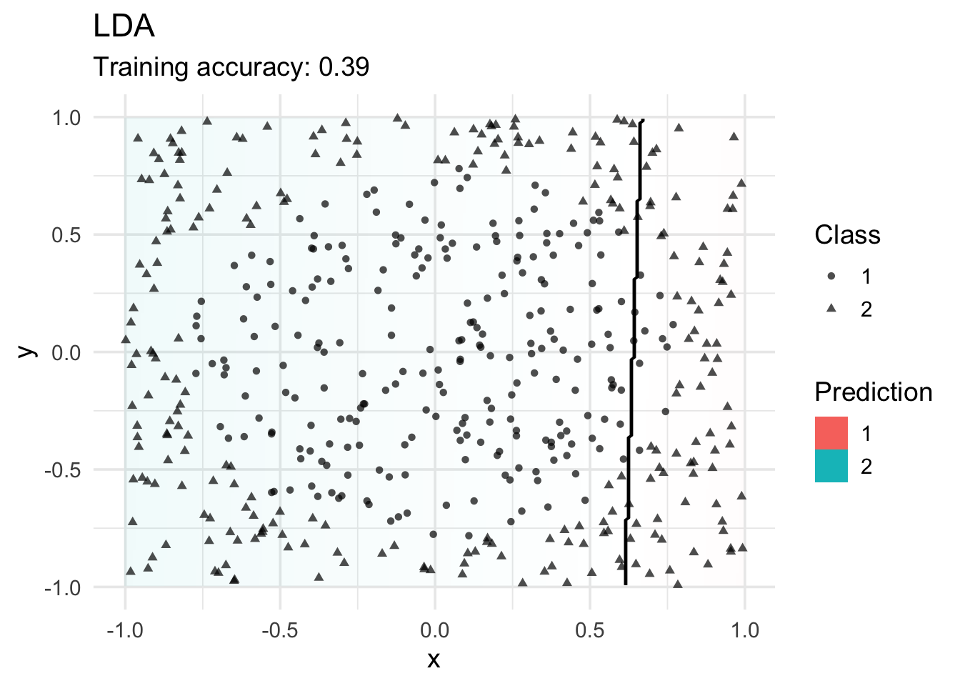

Logistic Regression (implemented in nnet)

Multinomial logistic regression is an extension of logistic regression to problems with more than two classes. It also tries to find a linear decision boundary.

model <- x |> nnet::multinom(class ~., data = _)

# weights:  4 (3 variable)
initial  value 346.573590 
final  value 346.308371 
converged

decisionplot(model, x, class_var = "class") + 
  labs(title = "Multinomial Logistic Regression",
       shape = "Class",
       fill = "Prediction")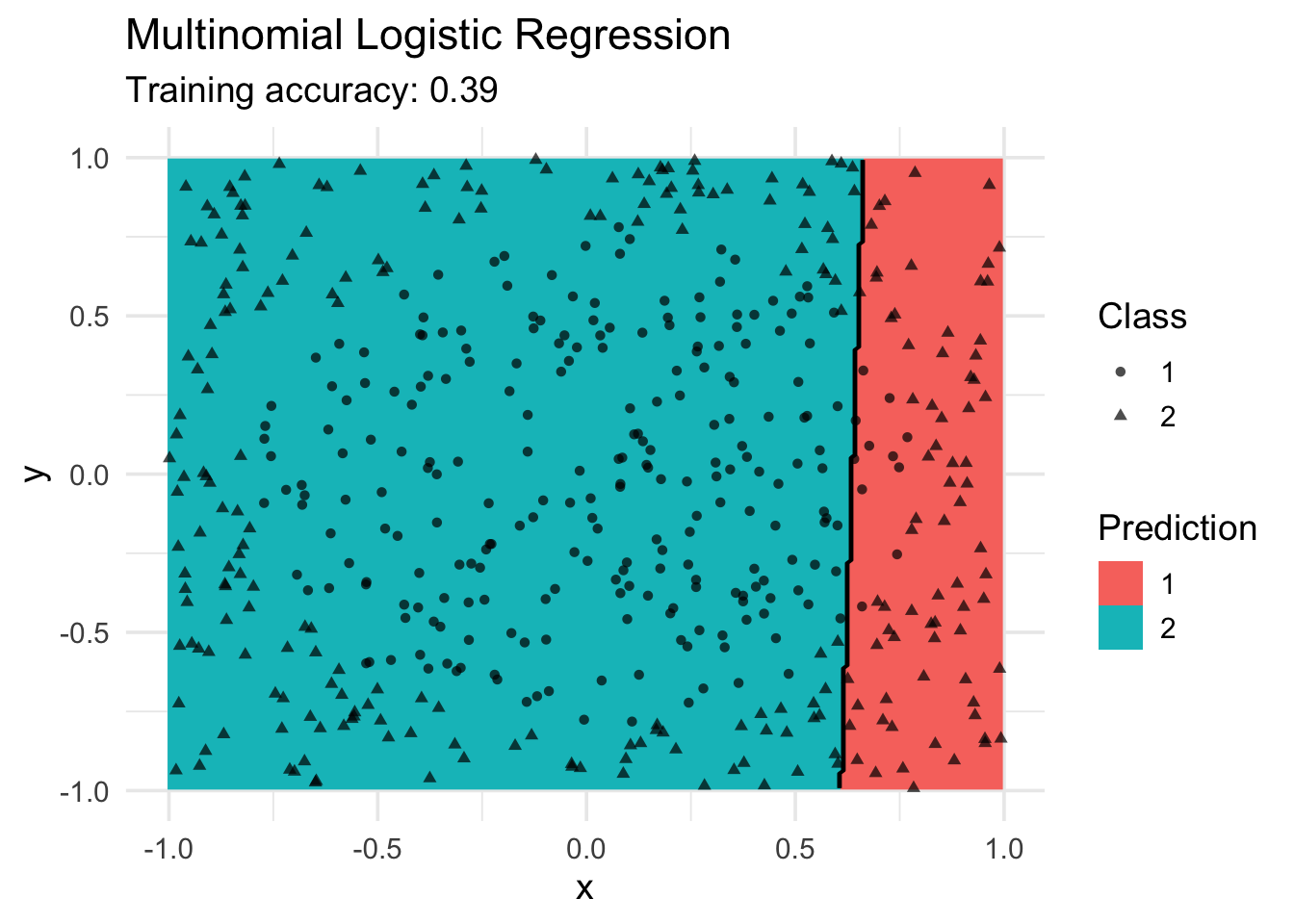

Decision Trees

model <- x |> rpart::rpart(class ~ ., data = _)
decisionplot(model, x, class_var = "class") + 
  labs(title = "CART",
       shape = "Class",
       fill = "Prediction")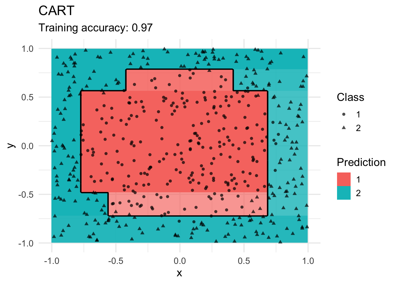

model <- x |> rpart::rpart(class ~ ., data = _,
  control = rpart.control(cp = 0.001, minsplit = 1))
decisionplot(model, x, class_var = "class") + 
  labs(title = "CART (overfitting)",
       shape = "Class",
       fill = "Prediction")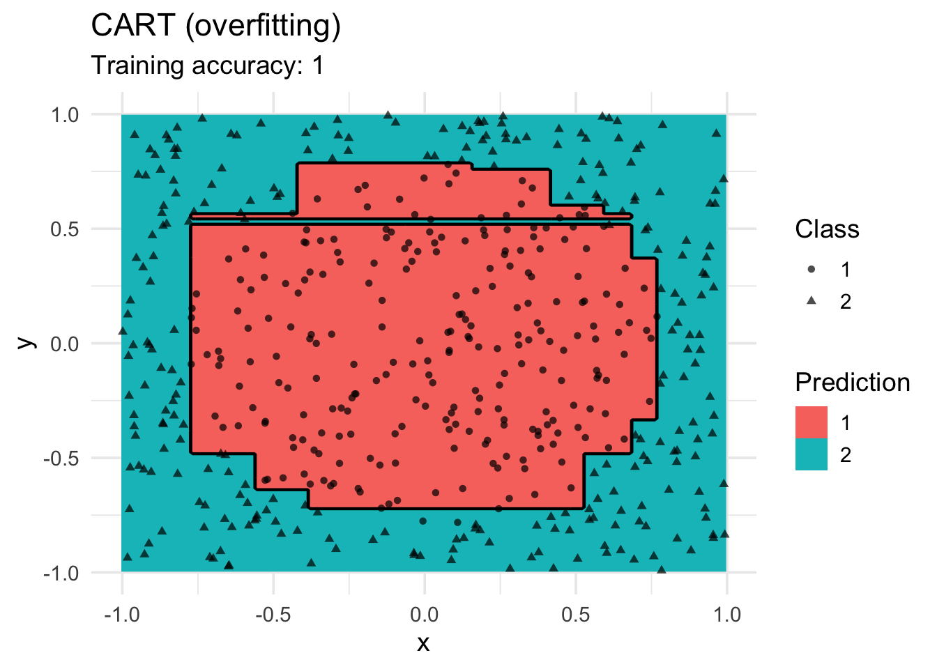

model <- x |> C50::C5.0(class ~ ., data = _)
decisionplot(model, x, class_var = "class") + 
  labs(title = "C5.0",
       shape = "Class",
       fill = "Prediction")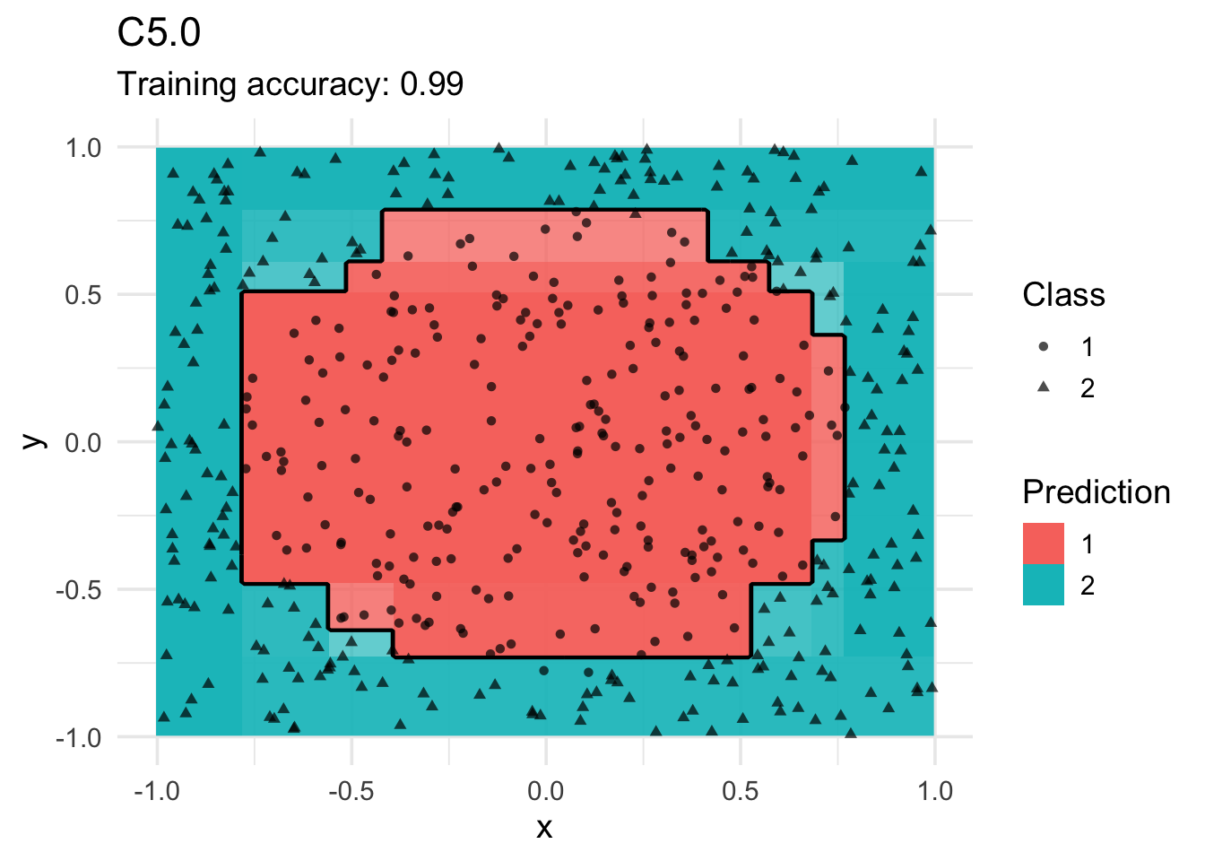

library(randomForest)
model <- x |> randomForest(class ~ ., data = _)
decisionplot(model, x, class_var = "class") + 
  labs(title = "Random Forest",
       shape = "Class",
       fill = "Prediction")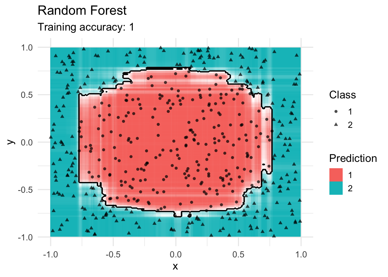

SVM

Linear SVM does not work for this data.

model <- x |> e1071::svm(class ~ ., data = _, kernel = "linear")
decisionplot(model, x, class_var = "class") + 
  labs(title = "SVM (linear kernel)",
       shape = "Class",
       fill = "Prediction")

Warning: Computation failed in `stat_contour()`
Caused by error in `if (zero_range(range)) ...`:
! missing value where TRUE/FALSE needed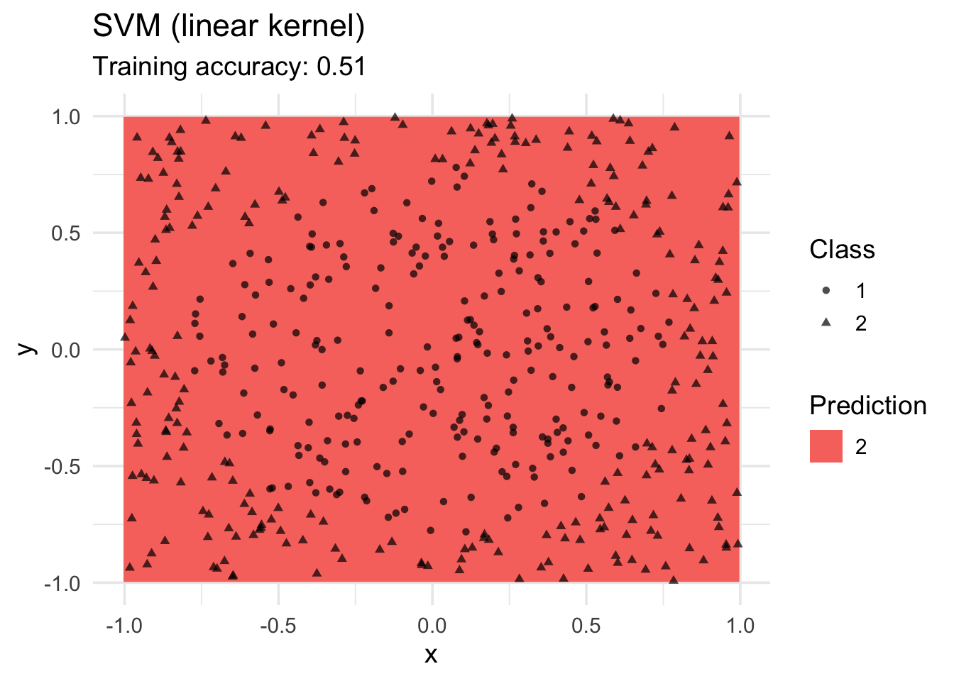

model <- x |> e1071::svm(class ~ ., data = _, kernel = "radial")
decisionplot(model, x, class_var = "class") + 
  labs(title = "SVM (radial kernel)",
       shape = "Class",
       fill = "Prediction")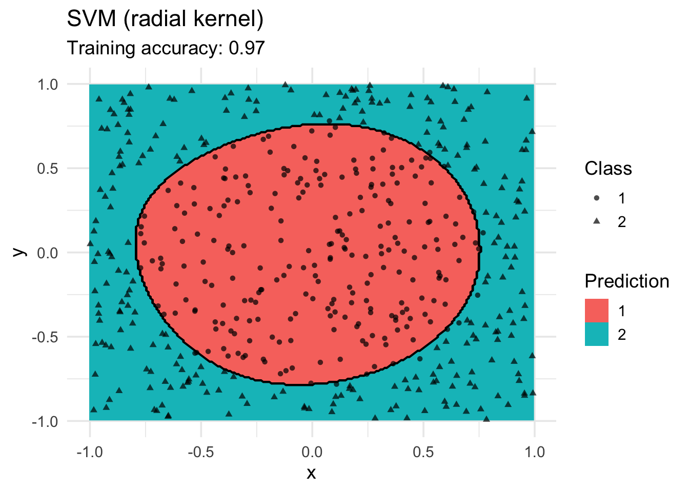

model <- x |> e1071::svm(class ~ ., data = _, kernel = "polynomial")
decisionplot(model, x, class_var = "class") + 
  labs(title = "SVM (polynomial kernel)",
       shape = "Class",
       fill = "Prediction")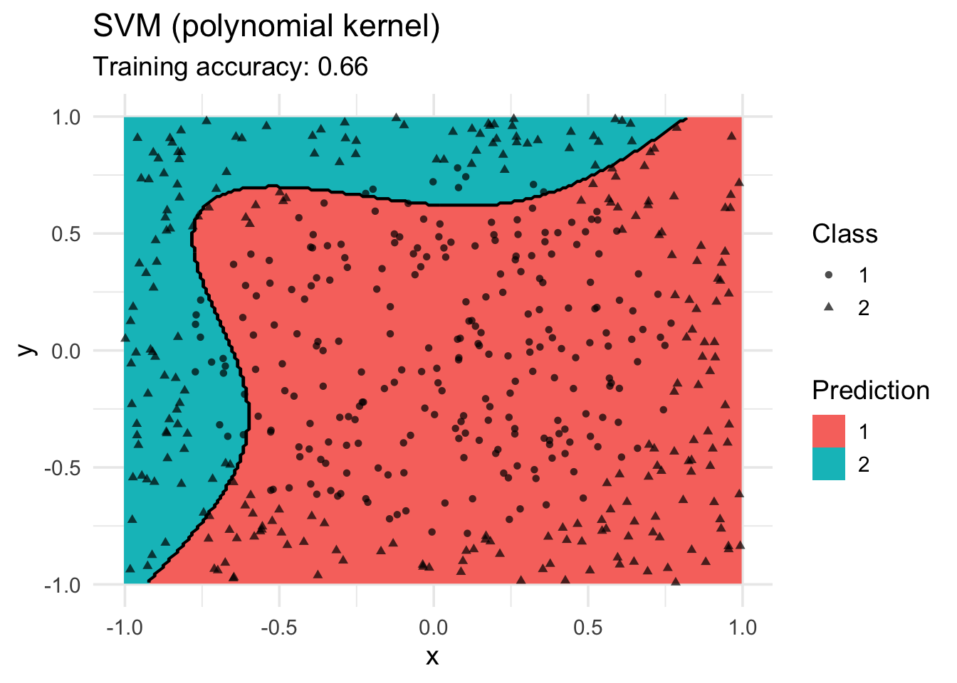

model <- x |> e1071::svm(class ~ ., data = _, kernel = "sigmoid")
decisionplot(model, x, class_var = "class") + 
  labs(title = "SVM (sigmoid kernel)",
       shape = "Class",
       fill = "Prediction")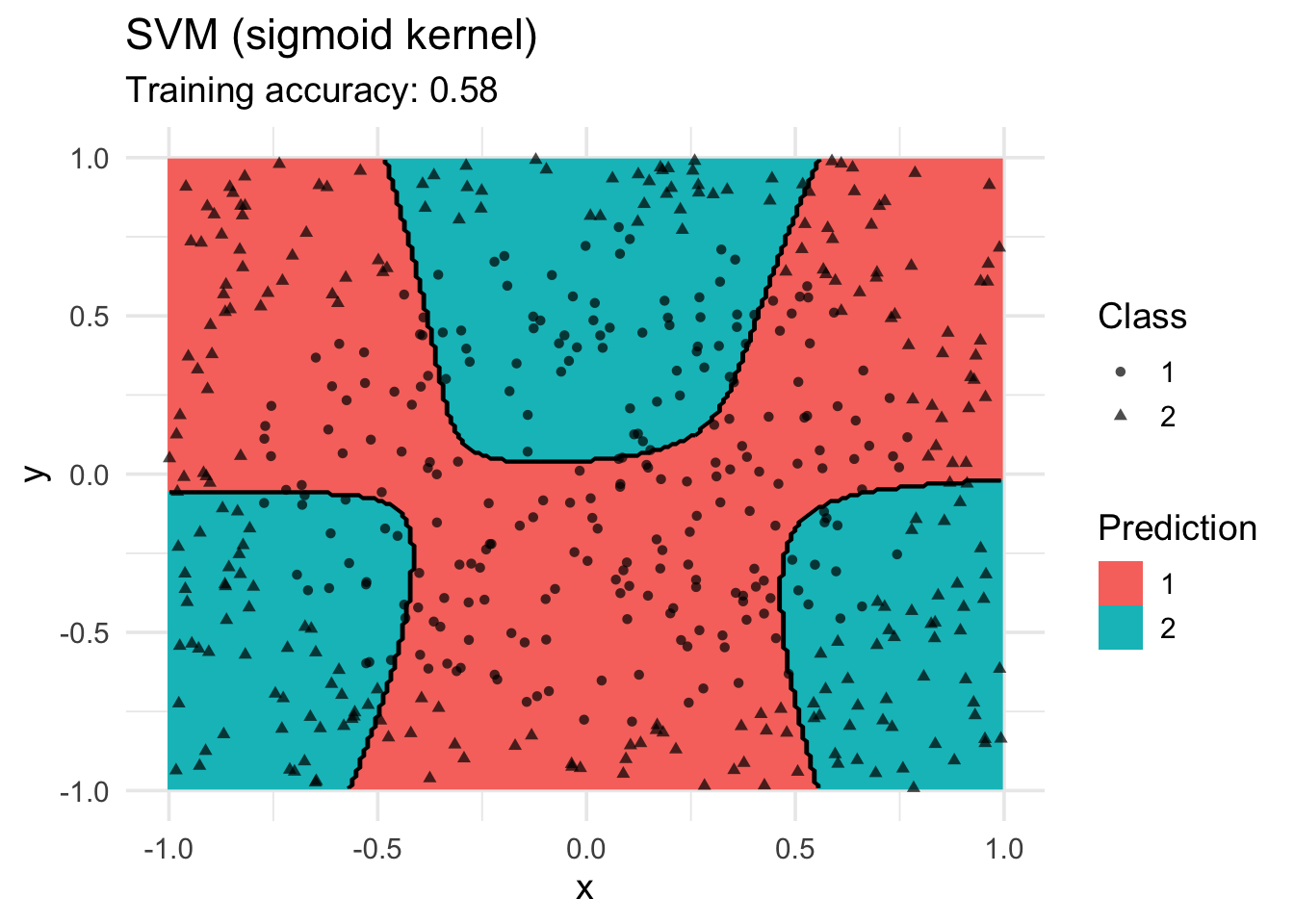

Single Layer Feed-forward Neural Networks

model <-x |> nnet::nnet(class ~ ., data = _, size = 1, trace = FALSE)
decisionplot(model, x, class_var = "class", 
  predict_type = c("class")) + 
  labs(title = "NN (1 neuron)",
       shape = "Class",
       fill = "Prediction")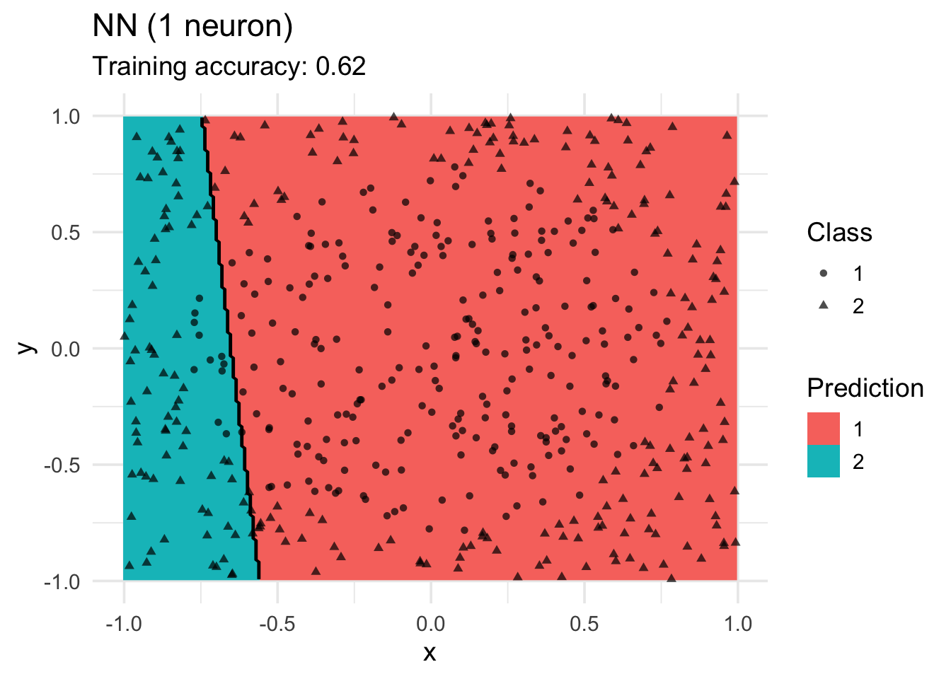

model <-x |> nnet::nnet(class ~ ., data = _, size = 2, trace = FALSE)
decisionplot(model, x, class_var = "class", 
  predict_type = c("class")) + 
  labs(title = "NN (2 neurons)",
       shape = "Class",
       fill = "Prediction")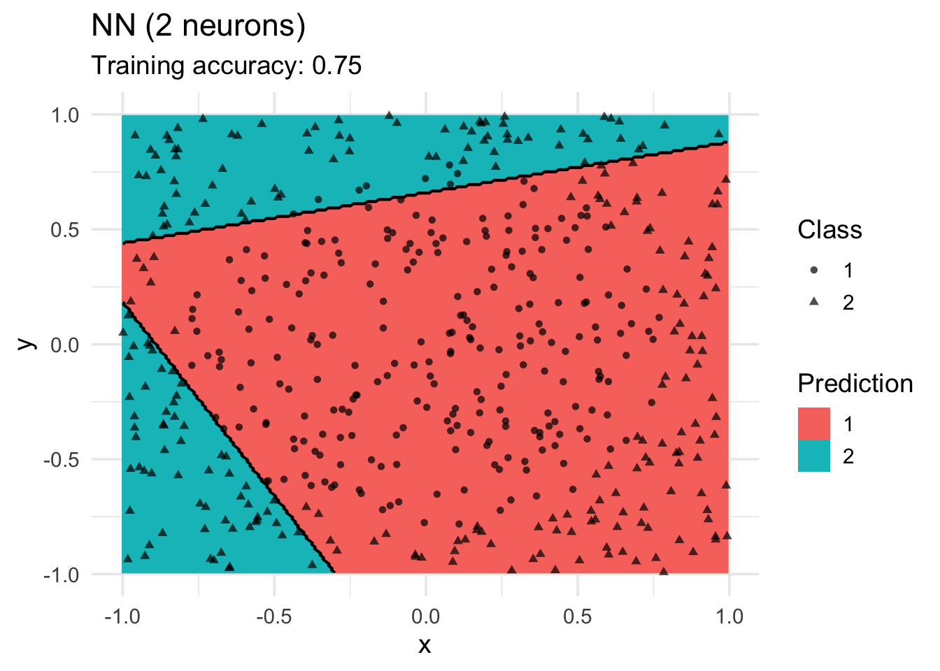

model <-x |> nnet::nnet(class ~ ., data = _, size = 4, trace = FALSE)
decisionplot(model, x, class_var = "class", 
  predict_type = c("class")) + 
  labs(title = "NN (4 neurons)",
       shape = "Class",
       fill = "Prediction")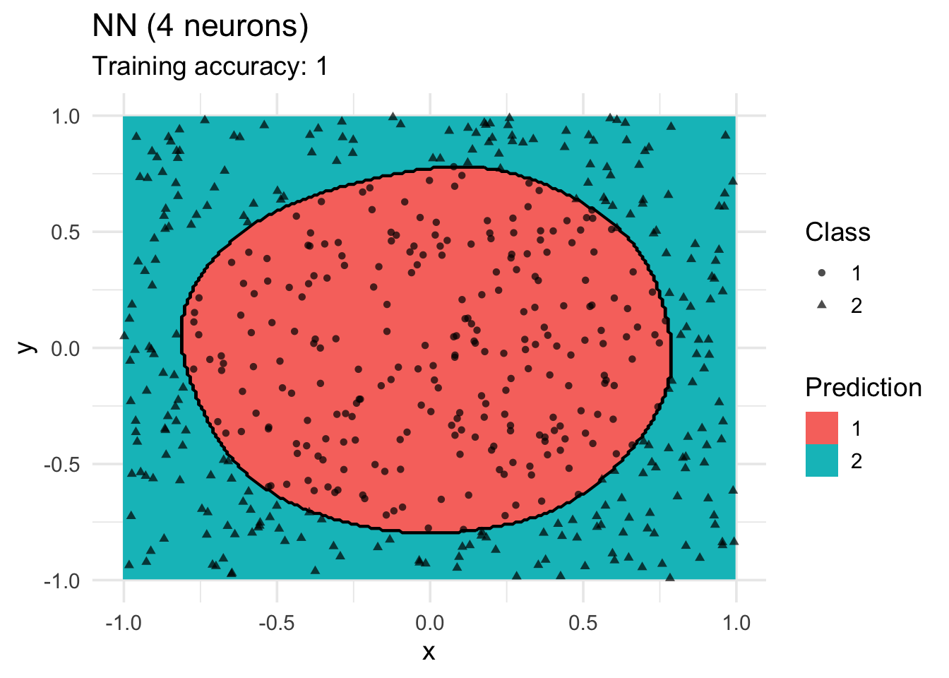

model <-x |> nnet::nnet(class ~ ., data = _, size = 10, trace = FALSE)
decisionplot(model, x, class_var = "class", 
  predict_type = c("class")) + 
  labs(title = "NN (10 neurons)",
       shape = "Class",
       fill = "Prediction")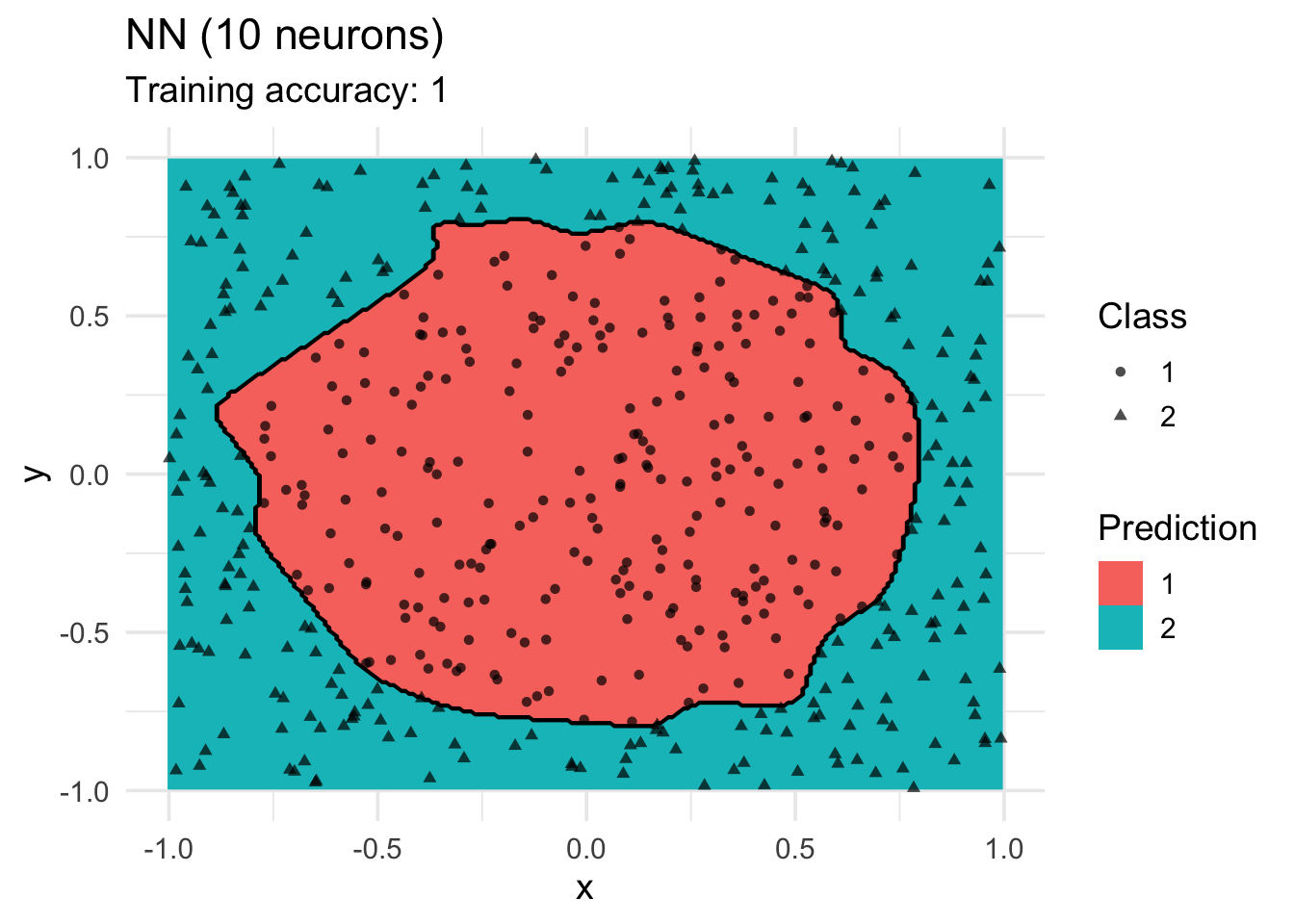

More Information on Classification with R

Package caret: http://topepo.github.io/caret/index.html
Tidymodels (machine learning with tidyverse): https://www.tidymodels.org/
R taskview on machine learning: http://cran.r-project.org/web/views/MachineLearning.html