library(pacman)

p_load(arules,
       arulesViz,
       dlookr,
tidyverse)Association Analysis in R
Goal
Practice R commands/methods for descriptive data analysis. If you are already familiar with some of the commands/methods, you can just practice the ones that are new to you.
Note: copying and pasting early in learning will not produce the results you are looking for, and will catch up to you eventually.
Submission
Please submit .r, .rmd, or .qmd files ONLY.
Overview
We will use packages:
arules: Provides the infrastructure for representing, manipulating and analyzing transaction data and patterns (frequent itemsets and association rules). Also provides C implementations of the association mining algorithms Apriori and Eclat. More see https://cran.r-project.org/web/packages/arules/arules.pdfarulesViz: Extends package ‘arules’ with various visualization techniques for association rules and itemsets. The package also includes several interactive visualizations for rule exploration. More see https://cran.r-project.org/web/packages/arulesViz/vignettes/arulesViz.pdfdplyr: A data manipulation grammar for working with data frame like objects, both in memory and out of memory. We used some of the command from this package, for more see https://cran.r-project.org/web/packages/dplyr/dplyr.pdf. Note that we are loading this package through thetidyverse
The Data Mining with R book used the Boston housing dataset as an example for association rule learning. Indeed, association rule learning can be used beyond transaction data mining.
Boston housing dataset description is at https://www.cs.toronto.edu/~delve/data/boston/bostonDetail.html
The 14 variables in this dataset include:
CRIM- per capita crime rate by townZN- proportion of residential land zoned for lots over 25,000 sq.ft.INDUS- proportion of non-retail business acres per town.CHAS- Charles River dummy variable (1 if tract bounds river; 0 otherwise)NOX- nitric oxides concentration (parts per 10 million)RM- average number of rooms per dwellingAGE- proportion of owner-occupied units built prior to 1940DIS- weighted distances to five Boston employment centresRAD- index of accessibility to radial highwaysTAX- full-value property-tax rate per $10,000PTRATIO- pupil-teacher ratio by townB - 1000(Bk - 0.63)^2where Bk is the proportion of blacks by townLSTAT - %lower status of the populationMEDV- Median value of owner-occupied homes in $1000’s
After going through this exercise, perform association rule learning on your dataset. If you have a text dataset, construct a document-term matrix from the text, then convert that to transaction data forma, you can treat the list of terms as items and mine association among the terms.
You want to explore different thresholds, use the interactive vis tools provided by arulesViz, and find and report at least two interesting association rules from your dataset.
Optional: If you would like to experience association rule mining using a transactional dataset, you can also try to use the Groceries dataset that comes with the arules package. Just say data(Groceries) to load the Groceries dataset after loading arules.
Load the data
data(Boston, package = "MASS")Transform variables
Association rules learning use categorical data. So the first step is transforming variables to factors.
Find classes of each of the column
The map() function is similar to lapply() but works more consistently with the tidyverse data structures:
map(Boston, class)$crim
[1] "numeric"
$zn
[1] "numeric"
$indus
[1] "numeric"
$chas
[1] "integer"
$nox
[1] "numeric"
$rm
[1] "numeric"
$age
[1] "numeric"
$dis
[1] "numeric"
$rad
[1] "integer"
$tax
[1] "numeric"
$ptratio
[1] "numeric"
$black
[1] "numeric"
$lstat
[1] "numeric"
$medv
[1] "numeric"All variables are ‘numeric’, really?
Use boxplot, histogram, and/or bar chart to review each of the variables
You will see chas, rad are likely categorical variables disguised as numerical variables
Show unique values in the variables chas and rad, confirming they are not continuous variables.
Boston |>
distinct(chas)
chas
1 0
2 1Boston |>
distinct(rad) rad
1 1
2 2
3 3
4 5
5 4
6 8
7 6
8 7
9 24Make these two variables factors
b <- Boston |>
  mutate(chas = factor(chas, labels = c("river", "noriver")),
         rad = factor(rad))
b |> head()
crim zn indus chas nox rm age dis rad tax ptratio black lstat
1 0.00632 18 2.31 river 0.538 6.575 65.2 4.0900 1 296 15.3 396.90 4.98
2 0.02731 0 7.07 river 0.469 6.421 78.9 4.9671 2 242 17.8 396.90 9.14
3 0.02729 0 7.07 river 0.469 7.185 61.1 4.9671 2 242 17.8 392.83 4.03
4 0.03237 0 2.18 river 0.458 6.998 45.8 6.0622 3 222 18.7 394.63 2.94
5 0.06905 0 2.18 river 0.458 7.147 54.2 6.0622 3 222 18.7 396.90 5.33
6 0.02985 0 2.18 river 0.458 6.430 58.7 6.0622 3 222 18.7 394.12 5.21
medv
1 24.0
2 21.6
3 34.7
4 33.4
5 36.2
6 28.7Bin all remaining numerical variables
Bin black first, to give it meaningful labels to aid interpretation:
b <- b |>
  mutate(black = binning(black, nbins = 4, labels = c(">31.5%", "18.5-31.5%", "8-18.5%", "<8%"), type = "equal"))
Now discretize all other numerical variables into 4 equal-width bins -- this is an arbitrary decision. Ideally expert domain knowledge should be consulted to bin, or try a few different ways, such as equal-depth. Also each variable can be binned differently.
bin <-function(x) binning(x, nbins = 4, labels=c("low", "medLow", "medHigh", "High"), type = "equal")Apply function bin on all numerical variables (-c() to exclude variables that have been converted to factors), then bind the newly cut variables back.
b <- b |>
  select(-c("chas", "rad", "black")) |>
  mutate_all(list(bin)) |>
  bind_cols(select(b, c("chas", "rad", "black")))
b |> head()
crim zn indus nox rm age dis tax ptratio lstat medv chas
1 low low low medLow medHigh medHigh medLow low medLow low medLow river
2 low low low low medHigh High medLow low medHigh low medLow river
3 low low low low medHigh medHigh medLow low medHigh low medHigh river
4 low low low low medHigh medLow medLow low medHigh low medHigh river
5 low low low low medHigh medHigh medLow low medHigh low medHigh river
6 low low low low medHigh medHigh medLow low medHigh low medHigh river
rad black
1 1 <8%
2 2 <8%
3 2 <8%
4 3 <8%
5 3 <8%
6 3 <8%dim(b)[1] 506 14b |> summary() crim
levels:c("low", "medLow", "medHigh", "High")
freq :c("491", " 10", " 2", " 3")
rate :c("0.970356", "0.019763", "0.003953", "0.005929")
zn
levels:c("low", "medLow", "medHigh", "High")
freq :c("429", " 32", " 16", " 29")
rate :c("0.84783", "0.06324", "0.03162", "0.05731")
indus
levels:c("low", "medLow", "medHigh", "High")
freq :c("202", "112", "165", " 27")
rate :c("0.39921", "0.22134", "0.32609", "0.05336")
nox
levels:c("low", "medLow", "medHigh", "High")
freq :c("200", "182", "100", " 24")
rate :c("0.39526", "0.35968", "0.19763", "0.04743")
rm
levels:c("low", "medLow", "medHigh", "High")
freq :c(" 8", "234", "236", " 28")
rate :c("0.01581", "0.46245", "0.46640", "0.05534")
age
levels:c("low", "medLow", "medHigh", "High")
freq :c(" 51", " 97", " 96", "262")
rate :c("0.1008", "0.1917", "0.1897", "0.5178")
dis
levels:c("low", "medLow", "medHigh", "High")
freq :c("305", "144", " 52", " 5")
rate :c("0.602767", "0.284585", "0.102767", "0.009881")
tax
levels:c("low", "medLow", "medHigh", "High")
freq :c("240", "128", " 1", "137")
rate :c("0.474308", "0.252964", "0.001976", "0.270751")
ptratio
levels:c("low", "medLow", "medHigh", "High")
freq :c(" 58", " 68", "171", "209")
rate :c("0.1146", "0.1344", "0.3379", "0.4130")
lstat
levels:c("low", "medLow", "medHigh", "High")
freq :c("243", "187", " 57", " 19")
rate :c("0.48024", "0.36957", "0.11265", "0.03755")
medv chas
levels:c("low", "medLow", "medHigh", "High") river :471
freq :c("116", "284", " 74", " 32") noriver: 35
rate :c("0.22925", "0.56126", "0.14625", "0.06324")
rad black
24 :132 levels:c(">31.5%", "18.5-31.5%", "8-18.5%", "<8%")
5 :115 freq :c(" 31", " 8", " 15", "452")
4 :110 rate :c("0.06126", "0.01581", "0.02964", "0.89328")
3 : 38
6 : 26
2 : 24
(Other): 61 Transform the dataframe b to a transactions dataset, where each row is described by a set of binary variables (this is “bitmap indexing” we learned in Chapter 4 in the textbook)
b <- as(b, "transactions")
#transactions data are often very large and sparse, directly looking at it won’t give your much information.You can see how the columns are constructed by using colnames(), or see a summary() of it. To see the records, use inspect(): inspect(b[1:9]) show the first 9 transactions. colnames(b) [1] "crim=low" "crim=medLow" "crim=medHigh" "crim=High"
[5] "zn=low" "zn=medLow" "zn=medHigh" "zn=High"
[9] "indus=low" "indus=medLow" "indus=medHigh" "indus=High"
[13] "nox=low" "nox=medLow" "nox=medHigh" "nox=High"
[17] "rm=low" "rm=medLow" "rm=medHigh" "rm=High"
[21] "age=low" "age=medLow" "age=medHigh" "age=High"
[25] "dis=low" "dis=medLow" "dis=medHigh" "dis=High"
[29] "tax=low" "tax=medLow" "tax=medHigh" "tax=High"
[33] "ptratio=low" "ptratio=medLow" "ptratio=medHigh" "ptratio=High"
[37] "lstat=low" "lstat=medLow" "lstat=medHigh" "lstat=High"
[41] "medv=low" "medv=medLow" "medv=medHigh" "medv=High"
[45] "chas=river" "chas=noriver" "rad=1" "rad=2"
[49] "rad=3" "rad=4" "rad=5" "rad=6"
[53] "rad=7" "rad=8" "rad=24" "black=>31.5%"
[57] "black=18.5-31.5%" "black=8-18.5%" "black=<8%" b |> summary()transactions as itemMatrix in sparse format with
506 rows (elements/itemsets/transactions) and
59 columns (items) and a density of 0.2372881
most frequent items:
crim=low chas=river black=<8% zn=low dis=low (Other)
491 471 452 429 305 4936
element (itemset/transaction) length distribution:
sizes
14
506
Min. 1st Qu. Median Mean 3rd Qu. Max.
14 14 14 14 14 14
includes extended item information - examples:
labels variables levels
1 crim=low crim low
2 crim=medLow crim medLow
3 crim=medHigh crim medHigh
includes extended transaction information - examples:
transactionID
1 1
2 2
3 3inspect(b[1:3]) #a transaction consists of a set of items and a transaction ID. Still have questions on transactions, check out another small example included at the end of this exercise. items transactionID
[1] {crim=low,
zn=low,
indus=low,
nox=medLow,
rm=medHigh,
age=medHigh,
dis=medLow,
tax=low,
ptratio=medLow,
lstat=low,
medv=medLow,
chas=river,
rad=1,
black=<8%} 1
[2] {crim=low,
zn=low,
indus=low,
nox=low,
rm=medHigh,
age=High,
dis=medLow,
tax=low,
ptratio=medHigh,
lstat=low,
medv=medLow,
chas=river,
rad=2,
black=<8%} 2
[3] {crim=low,
zn=low,
indus=low,
nox=low,
rm=medHigh,
age=medHigh,
dis=medLow,
tax=low,
ptratio=medHigh,
lstat=low,
medv=medHigh,
chas=river,
rad=2,
black=<8%} 3Show frequent items with minsup >= 0.3. Cex.names indicates the size of axis names:
Inspecting our results
Using arules
itemFrequencyPlot(b, support=0.3, cex.names=0.8)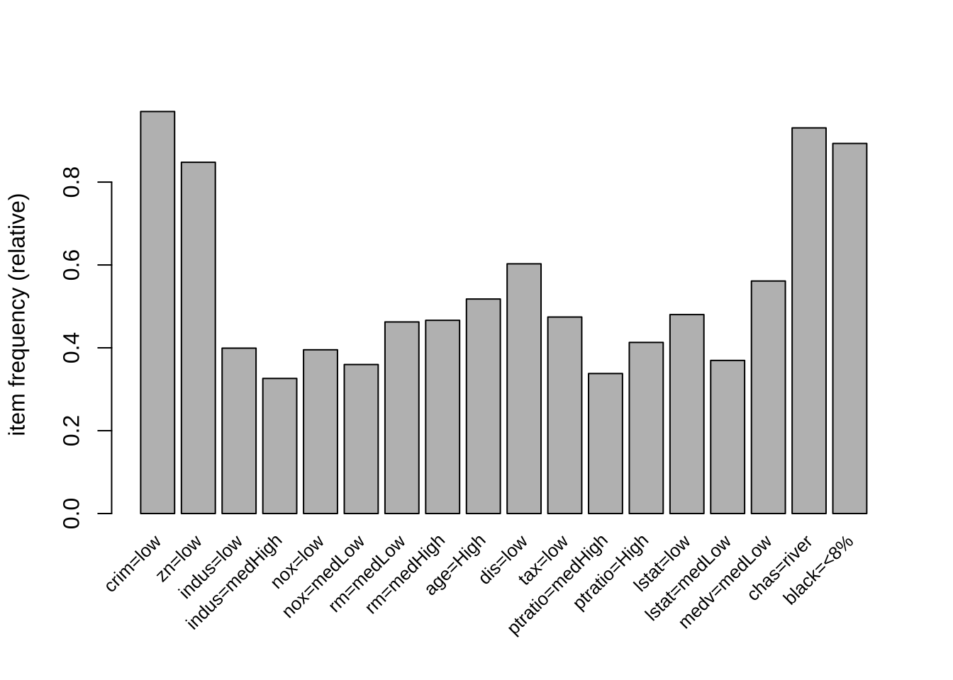
ars <- apriori(b, parameter = list(support = 0.025, confidence = 0.75))Apriori
Parameter specification:
confidence minval smax arem aval originalSupport maxtime support minlen
0.75 0.1 1 none FALSE TRUE 5 0.025 1
maxlen target ext
10 rules TRUE
Algorithmic control:
filter tree heap memopt load sort verbose
0.1 TRUE TRUE FALSE TRUE 2 TRUE
Absolute minimum support count: 12
set item appearances ...[0 item(s)] done [0.00s].
set transactions ...[59 item(s), 506 transaction(s)] done [0.00s].
sorting and recoding items ... [52 item(s)] done [0.00s].
creating transaction tree ... done [0.00s].
checking subsets of size 1 2 3 4 5 6 7 8 9 10Warning in apriori(b, parameter = list(support = 0.025, confidence = 0.75)):
Mining stopped (maxlen reached). Only patterns up to a length of 10 returned! done [0.02s].
writing ... [408638 rule(s)] done [0.02s].
creating S4 object ... done [0.17s].arsset of 408638 rules ars |> summary()set of 408638 rules
rule length distribution (lhs + rhs):sizes
1 2 3 4 5 6 7 8 9 10
4 293 3650 18932 53620 92554 103550 78411 41677 15947
Min. 1st Qu. Median Mean 3rd Qu. Max.
1.000 6.000 7.000 6.846 8.000 10.000
summary of quality measures:
support confidence coverage lift
Min. :0.02569 Min. :0.7500 Min. :0.02569 Min. : 0.7799
1st Qu.:0.02964 1st Qu.:0.9189 1st Qu.:0.02964 1st Qu.: 1.0743
Median :0.03755 Median :1.0000 Median :0.03953 Median : 1.6590
Mean :0.04857 Mean :0.9517 Mean :0.05150 Mean : 1.9759
3rd Qu.:0.05534 3rd Qu.:1.0000 3rd Qu.:0.05731 3rd Qu.: 2.4211
Max. :0.97036 Max. :1.0000 Max. :1.00000 Max. :19.4615
count
Min. : 13.00
1st Qu.: 15.00
Median : 19.00
Mean : 24.58
3rd Qu.: 28.00
Max. :491.00
mining info:
data ntransactions support confidence
b 506 0.025 0.75
call
apriori(data = b, parameter = list(support = 0.025, confidence = 0.75))Sub-setting by rules
Say we are interested in the association between pollution NOX and property value MEDV.
Find top 5 rules by confidence with medv = High attribute on the right side rhs
subset_result <- subset(ars, subset = rhs %in% "medv=High")
subset_result <- sort(subset_result, by = "confidence", decreasing = TRUE)
subset_result <- head(subset_result, n = 5)
inspect(subset_result)
lhs rhs support confidence coverage lift count
[1] {rm=High,
ptratio=low} => {medv=High} 0.02964427 1 0.02964427 15.8125 15
[2] {rm=High,
ptratio=low,
lstat=low} => {medv=High} 0.02964427 1 0.02964427 15.8125 15
[3] {rm=High,
ptratio=low,
black=<8%} => {medv=High} 0.02964427 1 0.02964427 15.8125 15
[4] {crim=low,
rm=High,
ptratio=low} => {medv=High} 0.02964427 1 0.02964427 15.8125 15
[5] {rm=High,
ptratio=low,
lstat=low,
black=<8%} => {medv=High} 0.02964427 1 0.02964427 15.8125 15Find top 5 rules by confidence with medv = low attribute on the right side rhs
subset_result <- subset(ars, subset = rhs %in% "medv=low")
subset_result <- sort(subset_result, by = "confidence", decreasing = TRUE)
subset_result <- head(subset_result, n = 5)
inspect(subset_result)
lhs rhs support confidence coverage lift count
[1] {nox=medHigh,
lstat=medHigh} => {medv=low} 0.05928854 1 0.05928854 4.362069 30
[2] {nox=medHigh,
lstat=medHigh,
rad=24} => {medv=low} 0.05928854 1 0.05928854 4.362069 30
[3] {nox=medHigh,
tax=High,
lstat=medHigh} => {medv=low} 0.05928854 1 0.05928854 4.362069 30
[4] {indus=medHigh,
nox=medHigh,
lstat=medHigh} => {medv=low} 0.05928854 1 0.05928854 4.362069 30
[5] {nox=medHigh,
ptratio=High,
lstat=medHigh} => {medv=low} 0.05928854 1 0.05928854 4.362069 30Use | (or) to include other conditions:
subset_result <- subset(ars, subset = rhs %in% "nox=High" | lhs %in% "nox=High")
subset_result <- sort(subset_result, by = "confidence", decreasing = TRUE)
subset_result <- head(subset_result, n = 5)
inspect(subset_result)
lhs rhs support confidence coverage lift
[1] {nox=High} => {indus=medHigh} 0.04743083 1 0.04743083 3.066667
[2] {nox=High} => {age=High} 0.04743083 1 0.04743083 1.931298
[3] {nox=High} => {dis=low} 0.04743083 1 0.04743083 1.659016
[4] {nox=High} => {zn=low} 0.04743083 1 0.04743083 1.179487
[5] {nox=High} => {crim=low} 0.04743083 1 0.04743083 1.030550
count
[1] 24
[2] 24
[3] 24
[4] 24
[5] 24 Showing top 5 rules by support with medv = High attribute on the right side rhs
subset_result <- subset(ars, subset = rhs %in% "medv=High")
subset_result <- sort(subset_result, by = "support", decreasing = TRUE)
subset_result <- head(subset_result, n = 5)
inspect(subset_result)
lhs rhs support confidence
[1] {rm=High} => {medv=High} 0.04743083 0.8571429
[2] {rm=High, lstat=low} => {medv=High} 0.04743083 0.8571429
[3] {rm=High, black=<8%} => {medv=High} 0.04743083 0.8571429
[4] {crim=low, rm=High} => {medv=High} 0.04743083 0.8571429
[5] {rm=High, lstat=low, black=<8%} => {medv=High} 0.04743083 0.8571429
coverage lift count
[1] 0.05533597 13.55357 24
[2] 0.05533597 13.55357 24
[3] 0.05533597 13.55357 24
[4] 0.05533597 13.55357 24
[5] 0.05533597 13.55357 24 Other ways to subset
Find rules generated from maximal/closed itemsets:
Maximal itemsets
subset_result <- subset(ars, subset = is.maximal(ars))
subset_result <- sort(subset_result, by = "confidence", decreasing = TRUE)
subset_result <- head(subset_result, n = 5)
inspect(subset_result)
lhs rhs support confidence
[1] {zn=low, lstat=medLow, chas=noriver} => {crim=low} 0.0256917 1
[2] {crim=low, lstat=medLow, chas=noriver} => {zn=low} 0.0256917 1
[3] {rm=medHigh, chas=noriver, black=<8%} => {crim=low} 0.0256917 1
[4] {crim=low, rm=medHigh, chas=noriver} => {black=<8%} 0.0256917 1
[5] {rm=medLow, ptratio=low, medv=medLow} => {crim=low} 0.0256917 1
coverage lift count
[1] 0.0256917 1.030550 13
[2] 0.0256917 1.179487 13
[3] 0.0256917 1.030550 13
[4] 0.0256917 1.119469 13
[5] 0.0256917 1.030550 13 Need to find freq itemsets to find closed itemsets:
freq.itemsets <- apriori(b, parameter = list(target = "frequent itemsets", support = 0.025))Apriori
Parameter specification:
confidence minval smax arem aval originalSupport maxtime support minlen
NA 0.1 1 none FALSE TRUE 5 0.025 1
maxlen target ext
10 frequent itemsets TRUE
Algorithmic control:
filter tree heap memopt load sort verbose
0.1 TRUE TRUE FALSE TRUE 2 TRUE
Absolute minimum support count: 12
set item appearances ...[0 item(s)] done [0.00s].
set transactions ...[59 item(s), 506 transaction(s)] done [0.00s].
sorting and recoding items ... [52 item(s)] done [0.00s].
creating transaction tree ... done [0.00s].
checking subsets of size 1 2 3 4 5 6 7 8 9 10Warning in apriori(b, parameter = list(target = "frequent itemsets", support =
0.025)): Mining stopped (maxlen reached). Only patterns up to a length of 10
returned! done [0.02s].
sorting transactions ... done [0.00s].
writing ... [106259 set(s)] done [0.01s].
creating S4 object ... done [0.01s].freq.itemsetsset of 106259 itemsets subset_result <- subset(ars, subset = is.closed(freq.itemsets))
subset_result <- sort(subset_result, by = "confidence", decreasing = TRUE)
subset_result <- head(subset_result, n = 5)
inspect(subset_result) lhs rhs support confidence coverage lift
[1] {rad=1} => {black=<8%} 0.03952569 1 0.03952569 1.119469
[2] {nox=High} => {indus=medHigh} 0.04743083 1 0.04743083 3.066667
[3] {nox=High} => {dis=low} 0.04743083 1 0.04743083 1.659016
[4] {nox=High} => {zn=low} 0.04743083 1 0.04743083 1.179487
[5] {rad=2} => {black=<8%} 0.04743083 1 0.04743083 1.119469
count
[1] 20
[2] 24
[3] 24
[4] 24
[5] 24 Find closed itemsets
closed = freq.itemsets[is.closed(freq.itemsets)]
closed |> summary()
set of 11351 itemsets
most frequent items:
crim=low black=<8% zn=low chas=river dis=low (Other)
9822 7839 7794 6833 4237 44615
element (itemset/transaction) length distribution:sizes
1 2 3 4 5 6 7 8 9 10
13 72 239 632 1309 2059 2346 1782 829 2070
Min. 1st Qu. Median Mean 3rd Qu. Max.
1.000 6.000 7.000 7.148 9.000 10.000
summary of quality measures:
support count
Min. :0.02569 Min. : 13.00
1st Qu.:0.03360 1st Qu.: 17.00
Median :0.04743 Median : 24.00
Mean :0.06915 Mean : 34.99
3rd Qu.:0.07708 3rd Qu.: 39.00
Max. :0.97036 Max. :491.00
includes transaction ID lists: FALSE
mining info:
data ntransactions support confidence
b 506 0.025 1
call
apriori(data = b, parameter = list(target = "frequent itemsets", support = 0.025))Find maximal itemsets
maximal = freq.itemsets[is.maximal(freq.itemsets)]
maximal |> summary()
set of 2949 itemsets
most frequent items:
crim=low chas=river zn=low black=<8% dis=low (Other)
2401 2247 2238 2093 1755 16939
element (itemset/transaction) length distribution:sizes
4 5 6 7 8 9 10
4 21 57 184 295 318 2070
Min. 1st Qu. Median Mean 3rd Qu. Max.
4.000 9.000 10.000 9.384 10.000 10.000
summary of quality measures:
support count
Min. :0.02569 Min. :13.00
1st Qu.:0.02569 1st Qu.:13.00
Median :0.02964 Median :15.00
Mean :0.03450 Mean :17.46
3rd Qu.:0.03755 3rd Qu.:19.00
Max. :0.14032 Max. :71.00
includes transaction ID lists: FALSE
mining info:
data ntransactions support confidence
b 506 0.025 1
call
apriori(data = b, parameter = list(target = "frequent itemsets", support = 0.025))Check shorter rules
subset_result <- subset(ars, subset = size(lhs) < 5 & size(lhs) > 1)
subset_result <- sort(subset_result, by = "support", decreasing = TRUE)
subset_result <- head(subset_result, n = 5)
inspect(subset_result)
lhs rhs support confidence coverage
[1] {chas=river, black=<8%} => {crim=low} 0.8083004 0.9784689 0.8260870
[2] {crim=low, black=<8%} => {chas=river} 0.8083004 0.9232506 0.8754941
[3] {crim=low, chas=river} => {black=<8%} 0.8083004 0.8969298 0.9011858
[4] {zn=low, chas=river} => {crim=low} 0.7569170 0.9623116 0.7865613
[5] {crim=low, zn=low} => {chas=river} 0.7569170 0.9251208 0.8181818
lift count
[1] 1.0083610 409
[2] 0.9918573 409
[3] 1.0040852 409
[4] 0.9917101 383
[5] 0.9938665 383 Note the above rules have high support and confidence but low lift.
subset_result <- subset(ars, subset = size(lhs) < 5 & size(lhs) > 1 & lift > 2)
subset_result <- sort(subset_result, by = "support", decreasing = TRUE)
subset_result <- head(subset_result, n = 5)
inspect(subset_result)
lhs rhs support confidence
[1] {nox=low, black=<8%} => {indus=low} 0.3221344 0.8150000
[2] {indus=low, black=<8%} => {nox=low} 0.3221344 0.8069307
[3] {crim=low, nox=low} => {indus=low} 0.3221344 0.8150000
[4] {crim=low, indus=low} => {nox=low} 0.3221344 0.8069307
[5] {crim=low, nox=low, black=<8%} => {indus=low} 0.3221344 0.8150000
coverage lift count
[1] 0.3952569 2.041535 163
[2] 0.3992095 2.041535 163
[3] 0.3952569 2.041535 163
[4] 0.3992095 2.041535 163
[5] 0.3952569 2.041535 163 arules compute many different kinds of interestMeasure besides support, confidence, and lift.
See the help page on interestMeasure for more examples.
Visualization of association rules
Static
plot(ars)To reduce overplotting, jitter is added! Use jitter = 0 to prevent jitter.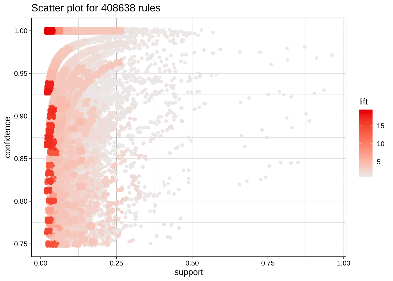
Interactive
Warning!!! : This interactive plot may crash R Studio. Save your project now before running the command below (or don’t run it…)
plot(ars, engine="interactive")Click the stop sign or the ESC key to terminate an interactive session.
You can filter your rules to a smaller set and then use the interactive exploration to identify interesting rules.
plot(ars, engine="htmlwidget")Grouped
somerules <- subset(ars, subset = size(lhs) > 1 & confidence > 0.90 & support > 0.5)

plot(somerules, method = "grouped")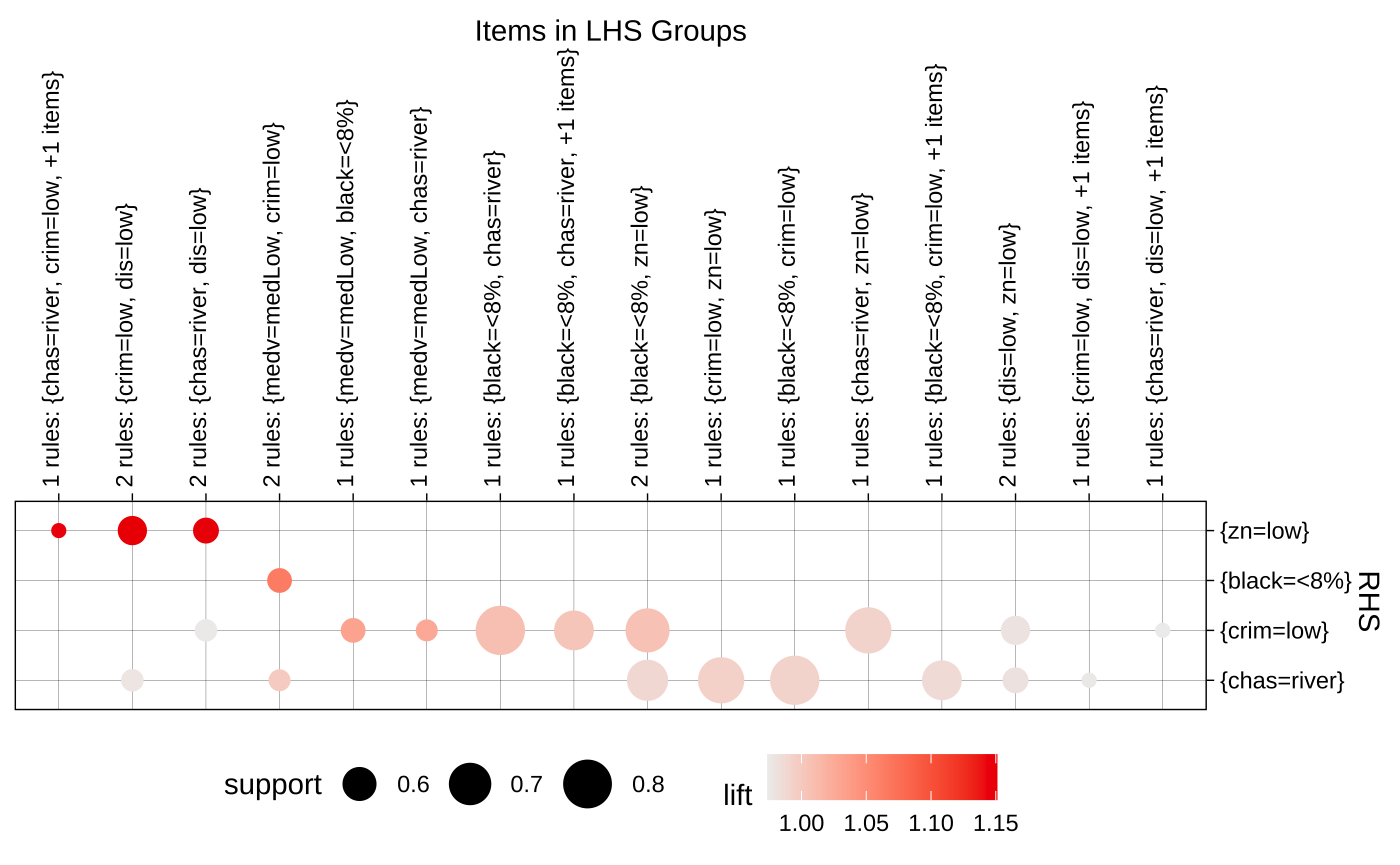
Matrix grouped plot
plot(somerules, method="matrix")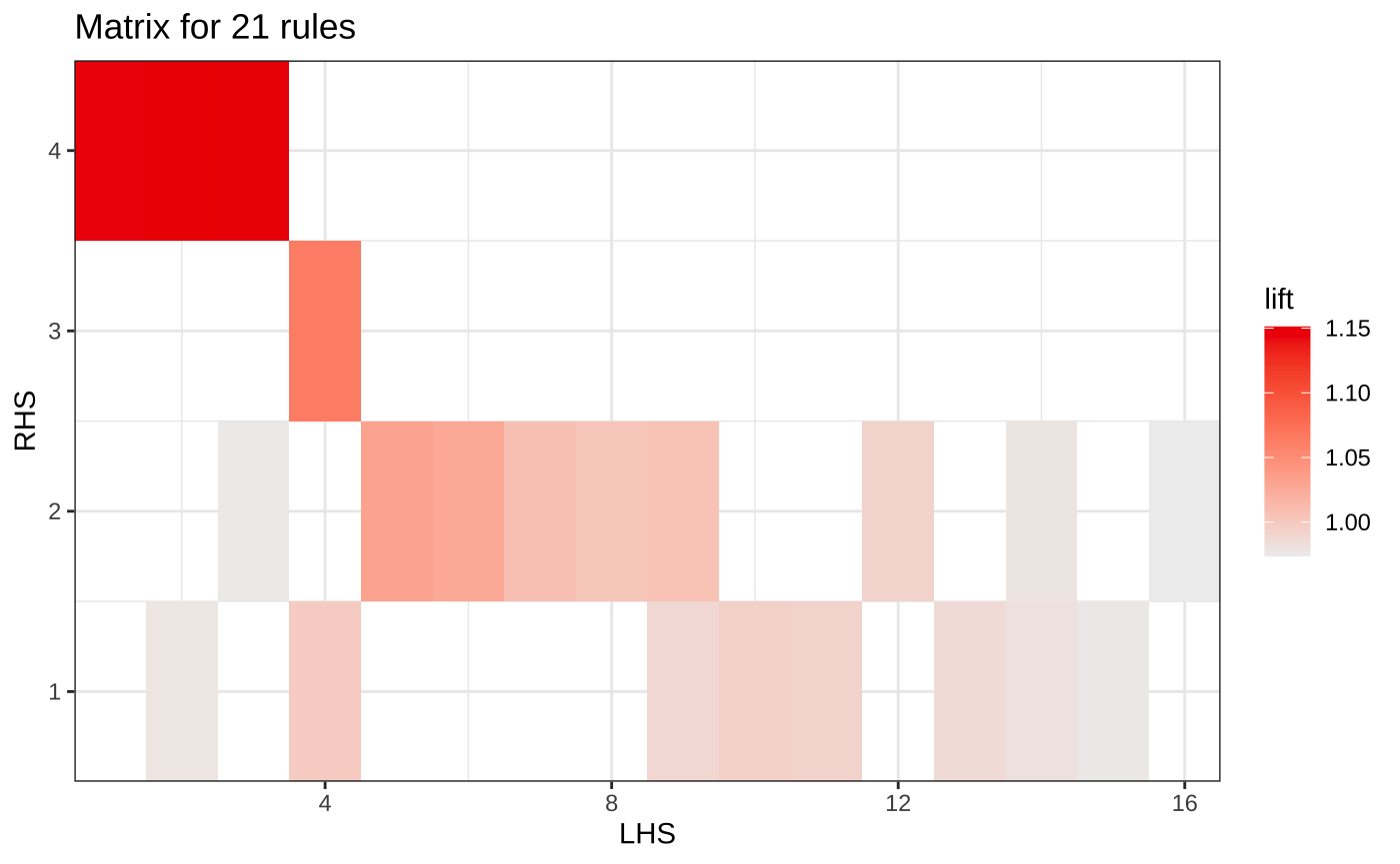
Graph (network) plot
plot(somerules, method = "graph")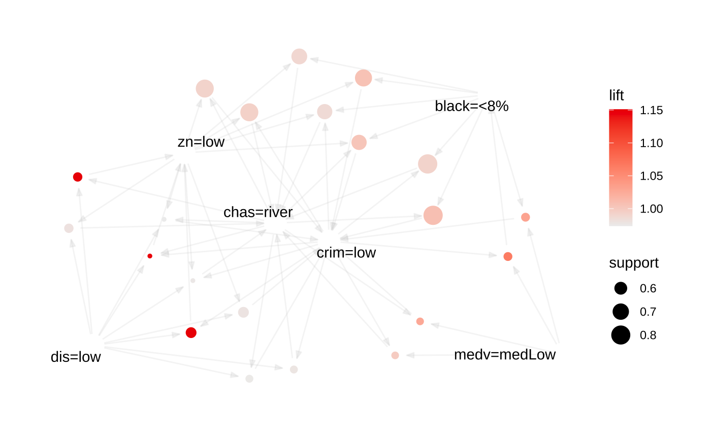
Interactive
plot(somerules, method = "graph", engine = "htmlwidget")Illustrate what is “transactions” data structure using a small example
Example
d <- data.frame(site = c("tucson", "phoenix"), season = c("spring", "summer"), price = c("high", "low"))
d
site season price
1 tucson spring high
2 phoenix summer lowConvert dataframe to transactions
d_t <-as(d, "transactions")Warning: Column(s) 1, 2, 3 not logical or factor. Applying default
discretization (see '? discretizeDF').d_ttransactions in sparse format with
2 transactions (rows) and
6 items (columns)Each row in the dataframe is converted to one transaction (2 transactions total).
What are the 6 items?
d_t |> summary()transactions as itemMatrix in sparse format with
2 rows (elements/itemsets/transactions) and
6 columns (items) and a density of 0.5
most frequent items:
site=phoenix site=tucson season=spring season=summer price=high
1 1 1 1 1
(Other)
1
element (itemset/transaction) length distribution:
sizes
3
2
Min. 1st Qu. Median Mean 3rd Qu. Max.
3 3 3 3 3 3
includes extended item information - examples:
labels variables levels
1 site=phoenix site phoenix
2 site=tucson site tucson
3 season=spring season spring
includes extended transaction information - examples:
transactionID
1 1
2 2Why density = 0.5?
Because the bitmap index is half empty:
| Site=t | Site=p | Season=sp | Season=su | Price=h | Price=l | |
| 1 | 1 | 1 | 1 | |||
| 2 | 1 | 1 | 1 |
Check out the transaction records
inspect(d_t[1:2]) items transactionID
[1] {site=tucson, season=spring, price=high} 1
[2] {site=phoenix, season=summer, price=low} 2 Each transaction has one itemset, and in this example, the itemset for transaction 1 is site=tucson, season=spring, price=high.
[ADVANCED]
Exercises on your data set:
Mine association rules from your dataset. Discuss a couple of interesting rules mined.