# Required packages
if (!require(pacman))
  install.packages("pacman")

pacman::p_load(tidymodels,
               tidyverse,
               ranger,
               randomForest,
               glmnet,
               gridExtra)

# Global ggplot theme
theme_set(theme_bw() + theme(legend.position = "top"))Regression in R
The following tutorial contains R examples for solving regression problems.
Regression is a modeling technique for predicting quantitative-valued target attributes. The goals for this tutorial are as follows: 1. To provide examples of using different regression methods from the tidymodels package. 2. To demonstrate the problem of model overfitting due to correlated attributes in the data. 3. To illustrate how regularization can be used to avoid model overfitting.
Read the step-by-step instructions below carefully. To execute the code, click on the corresponding cell and press the SHIFT-ENTER keys simultaneously.
Synthetic Data Generation
To illustrate how linear regression works, we first generate a random 1-dimensional vector of predictor variables, x, from a uniform distribution. The response variable y has a linear relationship with x according to the following equation: y = -3x + 1 + epsilon, where epsilon corresponds to random noise sampled from a Gaussian distribution with mean 0 and standard deviation of 1.
# Parameters
seed <- 1            # seed for random number generation
numInstances <- 200  # number of data instances

# Set seed
set.seed(seed)

# Generate data
X <- matrix(runif(numInstances), ncol=1)
y_true <- -3*X + 1
y <- y_true + matrix(rnorm(numInstances), ncol=1)

# Plot
ggplot() +
  geom_point(aes(x=X, y=y), color="black") +
  geom_line(aes(x=X, y=y_true), color="blue", linewidth=1) +
  ggtitle('True function: y = -3X + 1') +
  xlab('X') +
  ylab('y')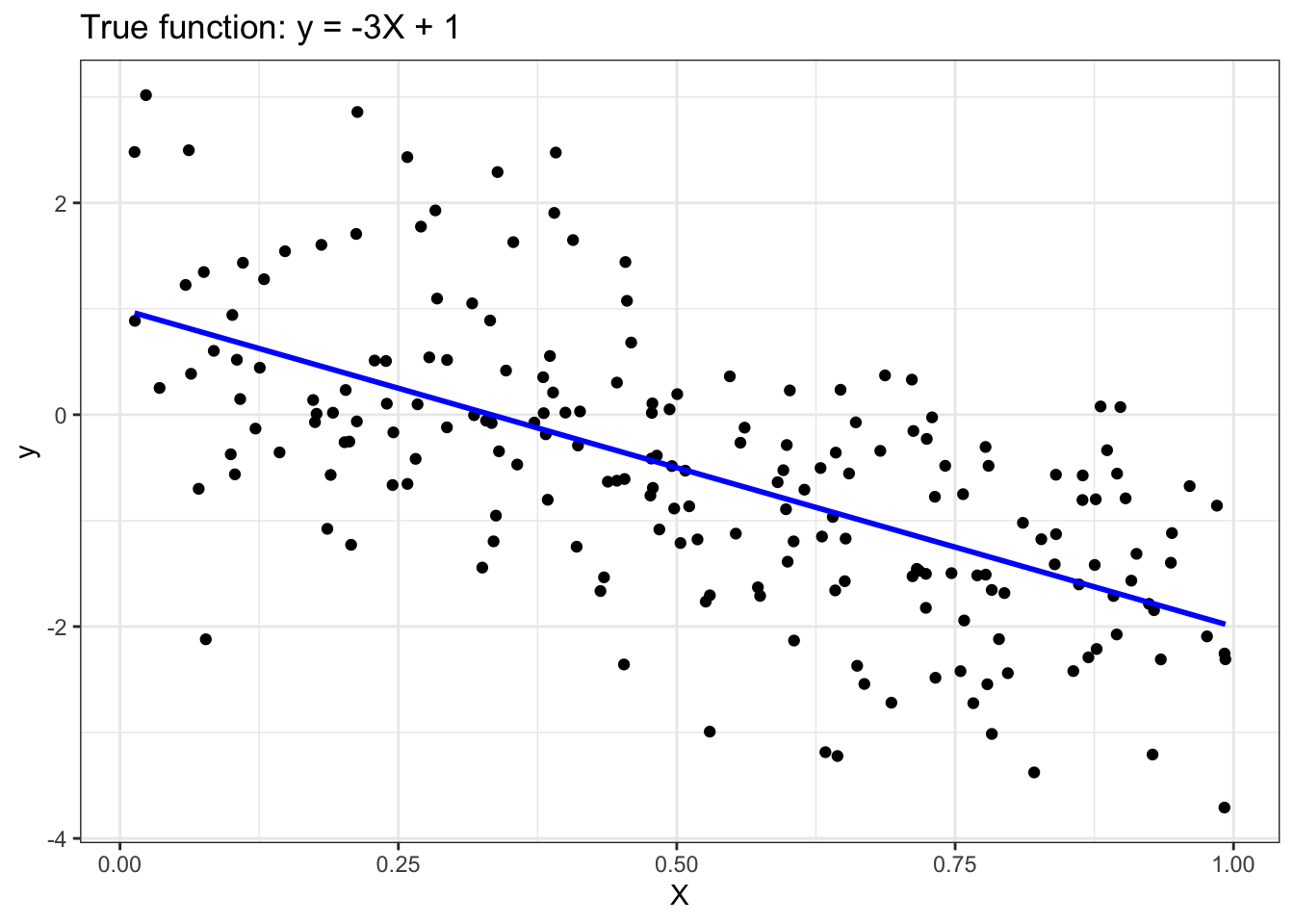
Multiple Linear Regression
In this example, we illustrate how to use Python scikit-learn package to fit a multiple linear regression (MLR) model. Given a training set \({X,y}\) MLR is designed to learn the regression function \(f(X,w) = X^T w + w_0\) by minimizing the following loss function given a training set \(\{X_i,y_i\}_{i=1}^N\):
\[ L(y,f(X,w)) = \sum_{i=1}^N \|y_i - X_i w - w_0\|^2, \]
where \(w\) (slope) and \(w_0\) (intercept) are the regression coefficients.
Given the input dataset, the following steps are performed: 1. Split the input data into their respective training and test sets. 2. Fit multiple linear regression to the training data. 3. Apply the model to the test data. 4. Evaluate the performance of the model. 5. Postprocessing: Visualizing the fitted model.
Step 1: Split Input Data into Training and Test Sets
# Train/test split
numTrain <- 20   # number of training instances
numTest <- numInstances - numTrain

set.seed(123) # For reproducibility

data <- tibble(X = X, y = y)

split_obj <- initial_split(data, prop = numTrain/numInstances)

# Extract train and test data
train_data <- training(split_obj)
test_data <- testing(split_obj)

# Extract X_train, X_test, y_train, y_test
X_train <- train_data$X
y_train <- train_data$y

X_test <- test_data$X
y_test <- test_data$y
Step 2: Fit Regression Model to Training Set
# Create a linear regression model specification
lin_reg_spec <- linear_reg() |>
  set_engine("lm")

# Fit the model to the training data
lin_reg_fit <- lin_reg_spec |>
  fit(y ~ X, data = train_data)
Step 3: Apply Model to the Test Set
# Apply model to the test set
y_pred_test <- predict(lin_reg_fit, new_data = test_data) |>
  pull(.pred)
Step 4: Evaluate Model Performance on Test Set
# Plotting true vs predicted values
ggplot() +
  geom_point(aes(x = as.vector(y_test), y = y_pred_test), color = 'black') +
  ggtitle('Comparing true and predicted values for test set') +
  xlab('True values for y') +
  ylab('Predicted values for y')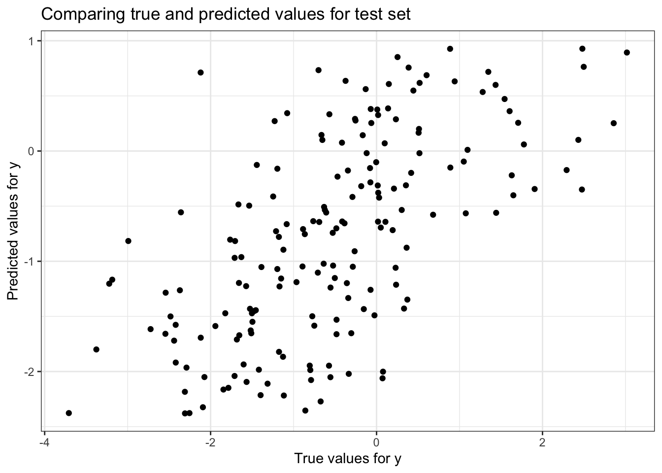
# Prepare data for yardstick evaluation
eval_data <- tibble(
  truth = as.vector(y_test),
  estimate = y_pred_test
)

# Model evaluation
rmse_value <- rmse(data = eval_data, truth = truth, estimate = estimate)
r2_value <- rsq(eval_data, truth = truth, estimate = estimate)

cat("Root mean squared error =", sprintf("%.4f", rmse_value$.estimate), "\n")
Root mean squared error = 1.0273 cat('R-squared =', sprintf("%.4f", r2_value$.estimate), "\n")R-squared = 0.3911 Step 5: Postprocessing
# Display model parameters
coef_values <- coef(lin_reg_fit$fit)  # Extract coefficients
slope <- coef_values["X"]
intercept <- coef_values["(Intercept)"]

cat("Slope =", slope, "\n")
Slope = -3.376872 cat("Intercept =", intercept, "\n")Intercept = 0.9723522 ### Step 4: Postprocessing
# Plot outputs
ggplot() +
geom_point(aes(x = as.vector(X_test), y = as.vector(y_test)), color = 'black') +
geom_line(aes(x = as.vector(X_test), y = y_pred_test), color = 'blue', linewidth = 1) +
ggtitle(sprintf('Predicted Function: y = %.2fX + %.2f', slope, intercept)) +
xlab('X') +
ylab('y')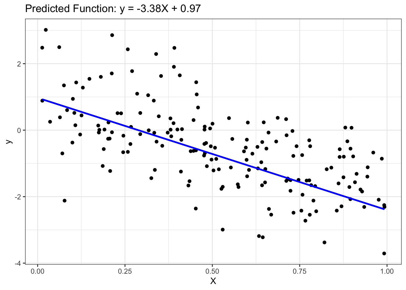
Effect of Correlated Attributes
In this example, we illustrate how the presence of correlated attributes can affect the performance of regression models. Specifically, we create 4 additional variables, X2, X3, X4, and X5 that are strongly correlated with the previous variable X created in Section 5.1. The relationship between X and y remains the same as before. We then fit y against the predictor variables and compare their training and test set errors.
First, we create the correlated attributes below.
# Generate the variables
set.seed(1)
X2 <- 0.5 * X + rnorm(numInstances, mean=0, sd=0.04)
X3 <- 0.5 * X2 + rnorm(numInstances, mean=0, sd=0.01)
X4 <- 0.5 * X3 + rnorm(numInstances, mean=0, sd=0.01)
X5 <- 0.5 * X4 + rnorm(numInstances, mean=0, sd=0.01)

# Create plots
plot1 <- ggplot() +
  geom_point(aes(X, X2), color='black') +
  xlab('X') + ylab('X2') +
  ggtitle(sprintf("Correlation between X and X2 = %.4f", cor(X[-c((numInstances-numTest+1):numInstances)], X2[-c((numInstances-numTest+1):numInstances)])))

plot2 <- ggplot() +
  geom_point(aes(X2, X3), color='black') +
  xlab('X2') + ylab('X3') +
  ggtitle(sprintf("Correlation between X2 and X3 = %.4f", cor(X2[-c((numInstances-numTest+1):numInstances)], X3[-c((numInstances-numTest+1):numInstances)])))

plot3 <- ggplot() +
  geom_point(aes(X3, X4), color='black') +
  xlab('X3') + ylab('X4') +
  ggtitle(sprintf("Correlation between X3 and X4 = %.4f", cor(X3[-c((numInstances-numTest+1):numInstances)], X4[-c((numInstances-numTest+1):numInstances)])))

plot4 <- ggplot() +
  geom_point(aes(X4, X5), color='black') +
  xlab('X4') + ylab('X5') +
  ggtitle(sprintf("Correlation between X4 and X5 = %.4f", cor(X4[-c((numInstances-numTest+1):numInstances)], X5[-c((numInstances-numTest+1):numInstances)])))

# Combine plots into a 2x2 grid
grid.arrange(plot1, plot2, plot3, plot4, ncol=2)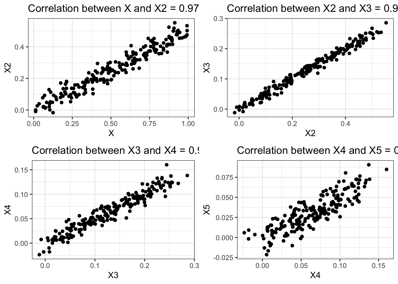
Next, we create 4 additional versions of the training and test sets. The first version, X_train2 and X_test2 have 2 correlated predictor variables, X and X2. The second version, X_train3 and X_test3 have 3 correlated predictor variables, X, X2, and X3. The third version have 4 correlated variables, X, X2, X3, and X4 whereas the last version have 5 correlated variables, X, X2, X3, X4, and X5.
# Split data into training and testing sets
train_indices <- 1:(numInstances - numTest)
test_indices <- (numInstances - numTest + 1):numInstances

# Create combined training and testing sets
X_train2 <- cbind(X[train_indices], X2[train_indices])
X_test2 <- cbind(X[test_indices], X2[test_indices])

X_train3 <- cbind(X[train_indices], X2[train_indices], X3[train_indices])
X_test3 <- cbind(X[test_indices], X2[test_indices], X3[test_indices])

X_train4 <- cbind(X[train_indices], X2[train_indices], X3[train_indices], X4[train_indices])
X_test4 <- cbind(X[test_indices], X2[test_indices], X3[test_indices], X4[test_indices])

X_train5 <- cbind(X[train_indices], X2[train_indices], X3[train_indices], X4[train_indices], X5[train_indices])
X_test5 <- cbind(X[test_indices], X2[test_indices], X3[test_indices], X4[test_indices], X5[test_indices])
Below, we train 4 new regression models based on the 4 versions of training and test data created in the previous step.
# Convert matrices to tibbles for training
train_data2 <- tibble(X1 = X_train2[,1], X2 = X_train2[,2], y = y_train)
train_data3 <- tibble(X1 = X_train3[,1], X2 = X_train3[,2], X3 = X_train3[,3], y = y_train)
train_data4 <- tibble(X1 = X_train4[,1], X2 = X_train4[,2], X3 = X_train4[,3], X4 = X_train4[,4], y = y_train)
train_data5 <- tibble(X1 = X_train5[,1], X2 = X_train5[,2], X3 = X_train5[,3], X4 = X_train5[,4], X5 = X_train5[,5], y = y_train)

# Train models
regr2_spec <- linear_reg() %>% set_engine("lm")
regr2_fit <- regr2_spec %>% fit(y ~ X1 + X2, data = train_data2)

regr3_spec <- linear_reg() %>% set_engine("lm")
regr3_fit <- regr3_spec %>% fit(y ~ X1 + X2 + X3, data = train_data3)

regr4_spec <- linear_reg() %>% set_engine("lm")
regr4_fit <- regr4_spec %>% fit(y ~ X1 + X2 + X3 + X4, data = train_data4)

regr5_spec <- linear_reg() %>% set_engine("lm")
regr5_fit <- regr5_spec %>% fit(y ~ X1 + X2 + X3 + X4 + X5, data = train_data5)
All 4 versions of the regression models are then applied to the training and test sets.
# Convert matrices to data.frames for predictions
new_train_data2 <- setNames(as.data.frame(X_train2), c("X1", "X2"))
new_test_data2 <- setNames(as.data.frame(X_test2), c("X1", "X2"))

new_train_data3 <- setNames(as.data.frame(X_train3), c("X1", "X2", "X3"))
new_test_data3 <- setNames(as.data.frame(X_test3), c("X1", "X2", "X3"))

new_train_data4 <- setNames(as.data.frame(X_train4), c("X1", "X2", "X3", "X4"))
new_test_data4 <- setNames(as.data.frame(X_test4), c("X1", "X2", "X3", "X4"))

new_train_data5 <- setNames(as.data.frame(X_train5), c("X1", "X2", "X3", "X4", "X5"))
new_test_data5 <- setNames(as.data.frame(X_test5), c("X1", "X2", "X3", "X4", "X5"))

# Predictions
y_pred_train2 <- predict(regr2_fit, new_data = new_train_data2)
y_pred_test2 <- predict(regr2_fit, new_data = new_test_data2)

y_pred_train3 <- predict(regr3_fit, new_data = new_train_data3)
y_pred_test3 <- predict(regr3_fit, new_data = new_test_data3)

y_pred_train4 <- predict(regr4_fit, new_data = new_train_data4)
y_pred_test4 <- predict(regr4_fit, new_data = new_test_data4)

y_pred_train5 <- predict(regr5_fit, new_data = new_train_data5)
y_pred_test5 <- predict(regr5_fit, new_data = new_test_data5)
For postprocessing, we compute both the training and test errors of the models. We can also show the resulting model and the sum of the absolute weights of the regression coefficients, i.e., \(\sum_{j=0}^d |w_j|\), where \(d\) is the number of predictor attributes.
# Extract coefficients and intercepts
get_coef <- function(model) {
  coef <- coefficients(model$fit)
  coef
}

# Calculate RMSE
calculate_rmse <- function(actual, predicted) {
  rmse <- sqrt(mean((actual - predicted)^2))
  rmse
}

results <- tibble(
  Model = c(sprintf("%.2f X + %.2f", get_coef(regr2_fit)['X1'], get_coef(regr2_fit)['(Intercept)']),
            sprintf("%.2f X + %.2f X2 + %.2f", get_coef(regr3_fit)['X1'], get_coef(regr3_fit)['X2'], get_coef(regr3_fit)['(Intercept)']),
            sprintf("%.2f X + %.2f X2 + %.2f X3 + %.2f", get_coef(regr4_fit)['X1'], get_coef(regr4_fit)['X2'], get_coef(regr4_fit)['X3'], get_coef(regr4_fit)['(Intercept)']),
            sprintf("%.2f X + %.2f X2 + %.2f X3 + %.2f X4 + %.2f", get_coef(regr5_fit)['X1'], get_coef(regr5_fit)['X2'], get_coef(regr5_fit)['X3'], get_coef(regr5_fit)['X4'], get_coef(regr5_fit)['(Intercept)'])),

  Train_error = c(calculate_rmse(y_train, y_pred_train2$.pred),
                  calculate_rmse(y_train, y_pred_train3$.pred),
                  calculate_rmse(y_train, y_pred_train4$.pred),
                  calculate_rmse(y_train, y_pred_train5$.pred)),

  Test_error = c(calculate_rmse(y_test, y_pred_test2$.pred),
                 calculate_rmse(y_test, y_pred_test3$.pred),
                 calculate_rmse(y_test, y_pred_test4$.pred),
                 calculate_rmse(y_test, y_pred_test5$.pred)),

  Sum_of_Absolute_Weights = c(sum(abs(get_coef(regr2_fit))),
                              sum(abs(get_coef(regr3_fit))),
                              sum(abs(get_coef(regr4_fit))),
                              sum(abs(get_coef(regr5_fit))))
)

# Plotting
ggplot(results, aes(x = Sum_of_Absolute_Weights)) +
  geom_line(aes(y = Train_error, color = "Train error"), linetype = "solid") +
  geom_line(aes(y = Test_error, color = "Test error"), linetype = "dashed") +
  labs(x = "Sum of Absolute Weights", y = "Error rate") +
  theme_minimal()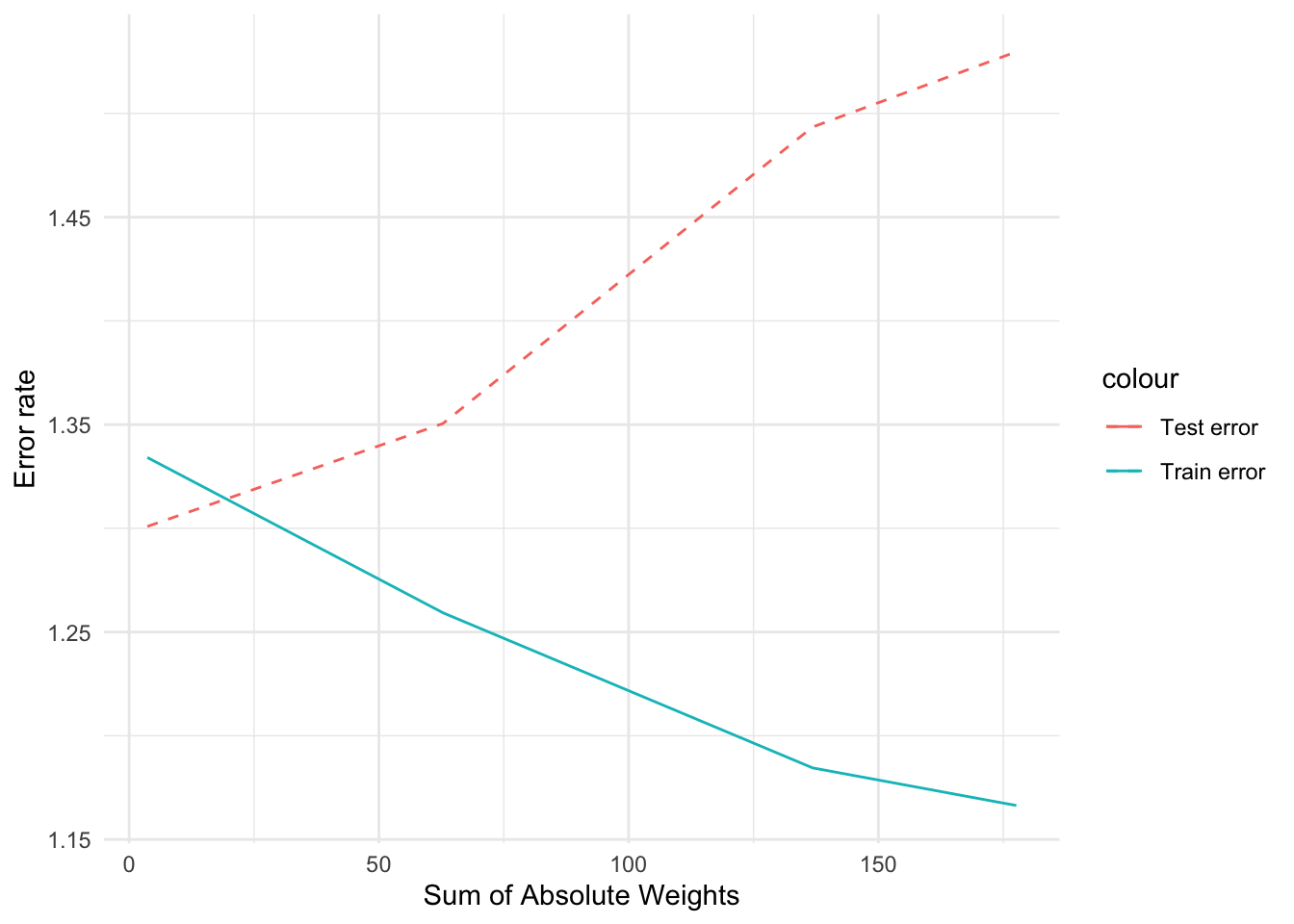
results# A tibble: 4 × 4
Model Train_error Test_error Sum_of_Absolute_Weig…¹
<chr> <dbl> <dbl> <dbl>
1 -0.53 X + -1.05 1.33 1.30 3.64
2 0.34 X + 20.99 X2 + -1.05 1.26 1.35 62.8
3 0.07 X + 22.72 X2 + -66.35 X3 +… 1.18 1.49 137.
4 -1.83 X + 22.46 X2 + -63.04 X3 … 1.17 1.53 178.
# ℹ abbreviated name: ¹Sum_of_Absolute_WeightsThe results above show that the first model, which fits y against X only, has the largest training error, but smallest test error, whereas the fifth model, which fits y against X and other correlated attributes, has the smallest training error but largest test error. This is due to a phenomenon known as model overfitting, in which the low training error of the model does not reflect how well the model will perform on previously unseen test instances. From the plot shown above, observe that the disparity between the training and test errors becomes wider as the sum of absolute weights of the model (which represents the model complexity) increases. Thus, one should control the complexity of the regression model to avoid the model overfitting problem.
Ridge Regression
Ridge regression is a variant of MLR designed to fit a linear model to the dataset by minimizing the following regularized least-square loss function:
\[ L_{\textrm{ridge}}(y,f(X,w)) = \sum_{i=1}^N \|y_i - X_iw - w_0\|^2 + \alpha \bigg[\|w\|^2 + w_0^2 \bigg], \]
where \(\alpha\) is the hyperparameter for ridge regression. Note that the ridge regression model reduces to MLR when \(\alpha = 0\). By increasing the value of \(\alpha\), we can control the complexity of the model as will be shown in the example below.
In the example shown below, we fit a ridge regression model to the previously created training set with correlated attributes. We compare the results of the ridge regression model against those obtained using MLR.
# Convert to data frame
train_data <- tibble(y = y_train, X_train5)
test_data <- tibble(y = y_test, X_test5)

# Set up a Ridge regression model specification
ridge_spec <- linear_reg(penalty = 0.4, mixture = 1) %>%
  set_engine("glmnet")

# Fit the model
ridge_fit <- ridge_spec %>%
  fit(y ~ ., data = train_data)

# Make predictions
y_pred_train_ridge <- predict(ridge_fit, new_data = train_data)$.pred
y_pred_test_ridge <- predict(ridge_fit, new_data = test_data)$.pred


# Make predictions
y_pred_train_ridge <- predict(ridge_fit, new_data = train_data)$.pred
y_pred_test_ridge <- predict(ridge_fit, new_data = train_data)$.pred

# Calculate RMSE
calculate_rmse <- function(actual, predicted) {
  rmse <- sqrt(mean((actual - predicted)^2))
  rmse
}

# Extract coefficients
ridge_coef <- coefficients(ridge_fit$fit)

model6 <- sprintf("%.2f X + %.2f X2 + %.2f X3 + %.2f X4 + %.2f X5 + %.2f",
                 ridge_coef[2], ridge_coef[3], ridge_coef[4],
                 ridge_coef[5], ridge_coef[6], ridge_coef[1])

values6 <- tibble(
  Model = model6,
  Train_error = calculate_rmse(y_train, y_pred_train_ridge),
  Test_error = calculate_rmse(y_test, y_pred_test_ridge),
  Sum_of_Absolute_Weights = sum(abs(ridge_coef))
)

# Combining the results
final_results <- bind_rows(results, values6)

final_results
# A tibble: 5 × 4
Model Train_error Test_error Sum_of_Absolute_Weig…¹
<chr> <dbl> <dbl> <dbl>
1 -0.53 X + -1.05 1.33 1.30 3.64
2 0.34 X + 20.99 X2 + -1.05 1.26 1.35 62.8
3 0.07 X + 22.72 X2 + -66.35 X3 +… 1.18 1.49 137.
4 -1.83 X + 22.46 X2 + -63.04 X3 … 1.17 1.53 178.
5 0.00 X + 0.00 X2 + 0.00 X3 + 0.… 1.35 1.29 8581.
# ℹ abbreviated name: ¹Sum_of_Absolute_WeightsBy setting an appropriate value for the hyperparameter, �, we can control the sum of absolute weights, thus producing a test error that is quite comparable to that of MLR without the correlated attributes.
Lasso Regression
One of the limitations of ridge regression is that, although it was able to reduce the regression coefficients associated with the correlated attributes and reduce the effect of model overfitting, the resulting model is still not sparse. Another variation of MLR, called lasso regression, is designed to produce sparser models by imposing an \(l_1\) regularization on the regression coefficients as shown below:
\[ L_{\textrm{lasso}}(y,f(X,w)) = \sum_{i=1}^N \|y_i - X_iw - w_0\|^2 + \alpha \bigg[ \|w\|_1 + |w_0|\bigg] \]
The example code below shows the results of applying lasso regression to the previously used correlated dataset.
# Define the lasso specification
lasso_spec <- linear_reg(penalty = 0.02, mixture = 1) %>%
  set_engine("glmnet")

# Ensure the data is combined correctly
train_data <- tibble(y = y_train, X1 = X_train5[,1], X2 = X_train5[,2],
                     X3 = X_train5[,3], X4 = X_train5[,4], X5 = X_train5[,5])

# Fit the model
lasso_fit <- lasso_spec %>%
  fit(y ~ ., data = train_data)

# Extract coefficients
lasso_coefs <- lasso_fit$fit$beta[,1]

# Predictions
y_pred_train_lasso <- predict(lasso_fit, new_data = train_data)$.pred
y_pred_test_lasso <- predict(lasso_fit, new_data = tibble(X1 = X_test5[,1], X2 = X_test5[,2],
                                                          X3 = X_test5[,3], X4 = X_test5[,4], X5 = X_test5[,5]))$.pred

# Create the model string
model7 <- sprintf("%.2f X + %.2f X2 + %.2f X3 + %.2f X4 + %.2f X5 + %.2f",
                  lasso_coefs[2], lasso_coefs[3], lasso_coefs[4],
                  lasso_coefs[5], lasso_coefs[6], lasso_fit$fit$a0[1])

values7 <- c(model7,
             sqrt(mean((y_train - y_pred_train_lasso)^2)),
             sqrt(mean((y_test - y_pred_test_lasso)^2)),
             sum(abs(lasso_coefs[-1])) + abs(lasso_fit$fit$a0[1]))

# Make the results tibble
lasso_results <- tibble(Model = "Lasso",
                        `Train error` = values7[2],
                        `Test error` = values7[3],
                        `Sum of Absolute Weights` = values7[4])

lasso_results
# A tibble: 1 × 4
Model `Train error` `Test error` `Sum of Absolute Weights`
<chr> <chr> <chr> <chr>
1 Lasso 1.22083472815552 1.36447668533408 0.750560758224512 Observe that the lasso regression model sets the coefficients for the correlated attributes, X2, X3, X4, and X5 to exactly zero unlike the ridge regression model. As a result, its test error is significantly better than that for ridge regression.
Hyperparameter Selection via Cross-Validation
While both ridge and lasso regression methods can potentially alleviate the model overfitting problem, one of the challenges is how to select the appropriate hyperparameter value, \(\alpha\). In the examples shown below, we demonstrate examples of using a 5-fold cross-validation method to select the best hyperparameter of the model. More details about the model selection problem and cross-validation method are described in Chapter 3 of the book.
In the first sample code below, we vary the hyperparameter \(\alpha\) for ridge regression to a range between 0.2 and 1.0. Using the RidgeCV() function, we can train a model with 5-fold cross-validation and select the best hyperparameter value.
# Combine training data
y_train <- as.vector(y_train)

train_data <- tibble(y = y_train, X1 = X_train5[,1], X2 = X_train5[,2],
                     X3 = X_train5[,3], X4 = X_train5[,4], X5 = X_train5[,5])

# Define recipe
recipe_obj <- recipe(y ~ ., data = train_data) %>%
  step_normalize(all_predictors()) |>
  prep()

# Define the ridge specification
ridge_spec <- linear_reg(penalty = tune(), mixture = 0) %>%
  set_engine("glmnet")

# Ridge workflow
ridge_wf <- workflow() |>
  add_model(ridge_spec) |>
  add_recipe(recipe_obj)

# Grid of alphas
alphas <- tibble(penalty = c(0.2, 0.4, 0.6, 0.8, 1.0))

# Tune
tune_results <-
  ridge_wf |>
  tune_grid(
  resamples = bootstraps(train_data, times = 5),
  grid = alphas
)


# Extract best parameters
best_params <- tune_results %>% select_best("rmse")

# Refit the model
ridge_fit <- ridge_spec %>%
  finalize_model(best_params) %>%
  fit(y ~ ., data = train_data)

# Extract coefficients
ridge_coefs <- ridge_fit$fit$beta[,1]

# Predictions
y_pred_train_ridge <- predict(ridge_fit, new_data = train_data)$.pred
y_pred_test_ridge <- predict(ridge_fit, new_data = tibble(X1 = X_test5[,1], X2 = X_test5[,2],
                                                          X3 = X_test5[,3], X4 = X_test5[,4], X5 = X_test5[,5]))$.pred

# Create the model string
model6 <- sprintf("%.2f X + %.2f X2 + %.2f X3 + %.2f X4 + %.2f X5 + %.2f",
                  ridge_coefs[2], ridge_coefs[3], ridge_coefs[4],
                  ridge_coefs[5], ridge_coefs[6], ridge_fit$fit$a0[1])

values6 <- c(model6,
             sqrt(mean((y_train - y_pred_train_ridge)^2)),
             sqrt(mean((y_test - y_pred_test_ridge)^2)),
             sum(abs(ridge_coefs[-1])) + abs(ridge_fit$fit$a0[1]))

# Make the results tibble
ridge_results <- tibble(Model = "RidgeCV",
                        `Train error` = values6[2],
                        `Test error` = values6[3],
                        `Sum of Absolute Weights` = values6[4])

cat("Selected alpha =", best_params$penalty, "\n")
Selected alpha = 1 all_results <- bind_rows(results, ridge_results)
all_results# A tibble: 5 × 7
Model Train_error Test_error Sum_of_Absolute_Weig…¹ `Train error` `Test error`
<chr> <dbl> <dbl> <dbl> <chr> <chr>
1 -0.5… 1.33 1.30 3.64 <NA> <NA>
2 0.34… 1.26 1.35 62.8 <NA> <NA>
3 0.07… 1.18 1.49 137. <NA> <NA>
4 -1.8… 1.17 1.53 178. <NA> <NA>
5 Ridg… NA NA NA 1.3309131350… 1.295979736…
# ℹ abbreviated name: ¹Sum_of_Absolute_Weights
# ℹ 1 more variable: `Sum of Absolute Weights` <chr>In this next example, we illustrate how to apply cross-validation to select the best hyperparameter value for fitting a lasso regression model.
set.seed(1234)

# Ensure y_train is a vector
y_train <- as.vector(y_train)

# Combine training data
train_data <- tibble(y = y_train, X1 = X_train5[,1], X2 = X_train5[,2],
                     X3 = X_train5[,3], X4 = X_train5[,4], X5 = X_train5[,5])

# Define recipe
recipe_obj_lasso <- recipe(y ~ ., data = train_data) %>%
  step_normalize(all_predictors()) |>
  prep()

# Define the lasso specification
lasso_spec <- linear_reg(penalty = tune(), mixture = 1) %>%
  set_engine("glmnet")

# Lasso workflow
lasso_wf <- workflow() |>
  add_recipe(recipe_obj_lasso)

# Lasso fit
lasso_fit <- lasso_wf |>
  add_model(lasso_spec) |>
  fit(data = train_data)

# Grid of alphas for Lasso
lambda_grid <- grid_regular(penalty(), levels = 50)

# Tune
tune_results_lasso <-
  tune_grid(lasso_wf |> add_model(lasso_spec),
  resamples = bootstraps(train_data, times = 5),
  grid = lambda_grid
)

# Extract best parameters for Lasso
best_params_lasso <- tune_results_lasso %>% select_best("rmse")

# Refit the model using Lasso
lasso_fit <- lasso_spec %>%
  finalize_model(best_params_lasso) %>%
  fit(y ~ ., data = train_data)

# Extract coefficients
lasso_coefs <- lasso_fit$fit$beta[,1]

# Predictions using Lasso
y_pred_train_lasso <- predict(lasso_fit, new_data = train_data)$.pred
y_pred_test_lasso <- predict(lasso_fit, new_data = tibble(X1 = X_test5[,1], X2 = X_test5[,2],
                                                          X3 = X_test5[,3], X4 = X_test5[,4], X5 = X_test5[,5]))$.pred

# Create the model string for Lasso
model7 <- sprintf("%.2f X + %.2f X2 + %.2f X3 + %.2f X4 + %.2f X5 + %.2f",
                  lasso_coefs[2], lasso_coefs[3], lasso_coefs[4],
                  lasso_coefs[5], lasso_coefs[6], lasso_fit$fit$a0[1])

values7 <- c(model7,
             sqrt(mean((y_train - y_pred_train_lasso)^2)),
             sqrt(mean((y_test - y_pred_test_lasso)^2)),
             sum(abs(lasso_coefs[-1])) + abs(lasso_fit$fit$a0[1]))

# Make the results tibble for Lasso
lasso_results <- tibble(Model = "LassoCV",
                        `Train error` = values7[2],
                        `Test error` = values7[3],
                        `Sum of Absolute Weights` = values7[4])

cat("Selected alpha for Lasso =", best_params_lasso$penalty, "\n")
Selected alpha for Lasso = 0.6250552 lasso_results# A tibble: 1 × 4
Model `Train error` `Test error` `Sum of Absolute Weights`
<chr> <chr> <chr> <chr>
1 LassoCV 1.34525910987747 1.28985807470116 0.750560758224512 Summary
This section presents example Python code for fitting linear regression models to a dataset. We also illustrate the problem of model overfitting and shows two alternative methods, called ridge and lasso regression, that can help alleviate such problem. While the model overfitting problem shown here is illustrated in the context of correlated attributes, the problem is more general and may arise due to other factors such as noise and other exceptional values in the data.